How to compute sky view factor from a surface model #

Problem statement #

Sky view factor is the fraction of the hemisphere above a point that is sky rather than building or terrain. It runs from 1 in the open to near 0 in a narrow courtyard, and it is the standard proxy for urban heat island intensity, diffuse daylight, night-time cooling and street-level thermal comfort.

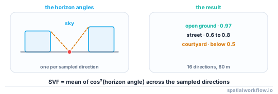
Computed from a surface model it is a horizon problem: in each of a set of directions, find the largest angle to the skyline, and integrate what is left. The two decisions that change the answer are how many directions you sample and how far you look, and neither has an obviously right value.

This guide computes SVF on a real derived DSM — 678 × 616 cells at 1 m over central The Hague, 19.5% built — and shows what the parameters do.

Quick answer #

import numpy as np

def sky_view_factor(dsm, res, n_dirs=16, max_dist=80):
    """Fraction of sky visible, from horizon angles in n_dirs directions."""
    steps = int(max_dist / res)
    horizon = np.zeros((n_dirs,) + dsm.shape, dtype="float32")
    for k in range(n_dirs):
        a = 2 * np.pi * k / n_dirs
        dx, dy = np.cos(a), -np.sin(a)
        best = np.zeros(dsm.shape, dtype="float32")
        for s in range(1, steps + 1):
            sx, sy = int(round(dx * s)), int(round(dy * s))
            if sx == 0 and sy == 0:
                continue
            shifted = np.roll(np.roll(dsm, -sy, axis=0), -sx, axis=1)
            best = np.maximum(best, (shifted - dsm) / (s * res))
        horizon[k] = np.arctan(best)
    return (np.cos(horizon) ** 2).mean(axis=0)

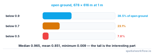
On the test DSM this gave a median SVF on open ground of 0.965, a mean of 0.851 and a minimum of 0.009, with 7.8% of open ground below 0.5 and 23.1% below 0.7.

Step-by-step solution #

1. Build or obtain a surface model #

A DSM from LiDAR is the right input. Without one, rasterise building heights onto a grid — that gives a built-form SVF that ignores trees, which is often what an urban morphology study wants anyway.

from rasterio.features import rasterize
from rasterio.transform import from_origin

dsm = rasterize(zip(b.geometry, b.height_m), out_shape=(h, w),
                transform=from_origin(minx, maxy, res, res), fill=0.0, dtype="float32")

2. Choose the resolution #

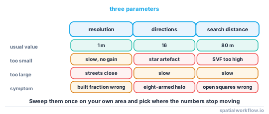
1 m is the usual compromise for street-level work. Coarser than about 2 m and narrow streets disappear; finer than 0.5 m and the cost grows without adding information, because building edges are not that sharp.

3. Choose the number of directions #

Eight is too few and shows a visible cross artefact; 16 is the common default; 32 is noticeably smoother and twice the cost. The difference between 16 and 32 is small in the open and larger in complex courtyards.

4. Choose the search distance #

Beyond a few times the tallest obstruction, further cells cannot raise the horizon. For a stock whose maximum height is 25 m, 80 m is generous. Too short a distance systematically overestimates SVF in wide streets with tall buildings at the end.

5. Use the correct integration formula #

For a horizon angle γ in each of n equal sectors, the standard estimator is SVF = (1/n) Σ cos²(γ). Using 1 − sin(γ) or the mean of cos(γ) are both different quantities, and all three appear in the literature — say which you used.

6. Decide where you are measuring #

SVF at ground level is what matters for thermal comfort and street daylight. SVF at roof level is what matters for solar. The same DSM gives both; the difference is whether you evaluate on built cells or only on open ground.

7. Report the distribution, not the mean #

The mean of 0.851 on the test tile is dominated by open ground. The interesting numbers are the fractions below thresholds — 7.8% below 0.5 and 23.1% below 0.7 — which locate the courtyards and narrow streets.

Code examples #

Example 1 — build the DSM and compute SVF end to end #

import numpy as np, geopandas as gpd, rasterio
from rasterio.features import rasterize
from rasterio.transform import from_origin

def dsm_from_buildings(b, res=1.0, height_col="height_m"):
    minx, miny, maxx, maxy = b.total_bounds
    w = int(np.ceil((maxx - minx) / res))
    h = int(np.ceil((maxy - miny) / res))
    tr = from_origin(minx, maxy, res, res)
    dsm = rasterize(((g, v) for g, v in zip(b.geometry, b[height_col])),
                    out_shape=(h, w), transform=tr, fill=0.0, dtype="float32")
    return dsm, tr

dsm, tr = dsm_from_buildings(b, res=1.0)
print(f"DSM {dsm.shape[1]} x {dsm.shape[0]} at 1.0 m, "
      f"built fraction {(dsm > 0).mean():.1%}, max height {dsm.max():.1f} m")

svf = sky_view_factor(dsm, res=1.0, n_dirs=16, max_dist=80)
ground = svf[dsm == 0]
print(f"SVF on open ground: min {ground.min():.3f}, median {np.median(ground):.3f}, "
      f"mean {ground.mean():.3f}, max {ground.max():.3f}")
for thr in (0.5, 0.7, 0.9):
    print(f"  below {thr}: {(ground < thr).mean():6.1%}")

DSM 678 x 616 at 1.0 m, built fraction 19.5%, max height 25.1 m
SVF on open ground: min 0.009, median 0.965, mean 0.851, max 1.000
  below 0.5:   7.8%
  below 0.7:  23.1%
  below 0.9:  39.5%

Example 2 — how the parameters change the answer #

import itertools, numpy as np

for n_dirs, max_dist in itertools.product((8, 16, 32), (40, 80, 160)):
    s = sky_view_factor(dsm, 1.0, n_dirs=n_dirs, max_dist=max_dist)
    g = s[dsm == 0]
    print(f"{n_dirs:3d} dirs, {max_dist:3d} m: median {np.median(g):.4f}, "
          f"mean {g.mean():.4f}, below 0.7 {(g < 0.7).mean():.2%}")

Run this once on your own study area and pick the point where the numbers stop moving. Reporting the parameters is as important as reporting the values.

Example 3 — write it out, and sample it at points #

import rasterio, geopandas as gpd

profile = {"driver": "GTiff", "height": svf.shape[0], "width": svf.shape[1],
           "count": 1, "dtype": "float32", "crs": b.crs, "transform": tr,
           "compress": "deflate", "predictor": 3, "tiled": True}
with rasterio.open("svf.tif", "w", **profile) as dst:
    dst.write(svf.astype("float32"), 1)
    dst.descriptions = ("sky view factor",)
    dst.update_tags(METHOD="16 directions, 80 m, cos^2 integration",
                    DSM="buildings rasterised at 1 m, no vegetation")

with rasterio.open("svf.tif") as src:
    pts["svf"] = [v[0] for v in src.sample(zip(pts.geometry.x, pts.geometry.y))]

Putting the method in the tags matters more here than for most rasters, because three different SVF definitions are in common use and the values are not comparable between them.

Explanation #

Why the cos² formula #

For an unobstructed hemisphere, the fraction of sky in a sector with horizon angle γ is cos²(γ) under the assumption of uniform sky radiance weighted by the cosine of the zenith angle — which is the assumption that makes SVF proportional to diffuse irradiance received. Averaging over equal-azimuth sectors gives the whole-hemisphere estimate. Other definitions exist, including the simpler 1 − sin(γ), which corresponds to a uniform radiance sky with no cosine weighting.

Why the direction count shows up as a cross #

With eight directions the sampled azimuths are the cardinal and diagonal ones, so a building corner that blocks the sky between two sampled directions is missed entirely. The artefact looks like a faint eight-armed star around obstructions. Sixteen directions reduces it below the noise for most purposes.

Why the search distance matters more than it looks #

An obstruction at distance d and height h subtends atan(h/d). At 80 m a 25 m building subtends 17°, which removes about 9% of the sky in that sector — not negligible. Cutting the search at 40 m in a stock with 25 m buildings systematically raises SVF in open squares surrounded by tall blocks, which are exactly the locations a heat study cares about.

Why the shift-and-compare implementation is fast #

Rolling the whole array by a fixed offset and taking a maximum is vectorised over every cell at once, so the cost is n_dirs × steps array operations rather than a per-cell ray cast. For a 678 × 616 grid with 16 directions and 80 steps that is 1,280 array passes, which runs in seconds. Note that np.roll wraps at the edges, so the outer max_dist metres of the result are contaminated — crop them, or pad the DSM first.

Edge cases or notes #

• np.roll wraps. Pad the DSM by max_dist and crop the result.
• Vegetation is usually the dominant obstruction at street level and is absent from a building-only DSM.
• Terrain matters in hilly cities and belongs in the same surface.
• Evaluate on open ground. SVF on a rooftop cell is a different quantity.
• Nodata in a DSM propagates. Fill before computing.
• Report the definition. cos², 1 − sin and continuous integration give different numbers.
• Anisotropic SVF exists for directional sky radiance; this is the isotropic version.
• A coarse DSM closes narrow streets. Check the built fraction at your resolution.

Internal links #

• How to compute building shadows for a given time in Python — direct rather than diffuse light
• How to estimate rooftop solar potential in Python — where roof-level SVF is the shading correction
• How to extrude building footprints into 3D in Python — producing the input
• LiDAR surfaces explained: DSM, DTM and CHM — the measured DSM
• How to calculate a viewshed in Python — the same horizon problem, one direction at a time
• How to rasterize a vector layer in Python — building the DSM
• How to create a hillshade in Python — another angle-from-a-surface calculation
• How to test whether a window can see a landmark — line of sight in 3D

FAQ #

What is sky view factor? #

The fraction of the sky hemisphere visible from a point: 1 in the open, near 0 in a narrow courtyard. It is the standard proxy for diffuse daylight and night-time cooling.

How do I compute it from a DSM? #

Find the maximum horizon angle in each of n directions, then average cos² of those angles across the directions.

How many directions should I use? #

Sixteen is the common default. Eight produces a visible star artefact around obstructions; thirty-two is smoother and twice the cost.

How far should I search? #

Far enough that further cells cannot raise the horizon — roughly three times the tallest obstruction. For 25 m buildings, 80 m is generous.

What resolution do I need? #

About 1 m for street-level work. At 2 m or coarser, narrow streets close up and the SVF is wrong where it matters most.

Why do my edges look wrong? #

np.roll wraps around the array. Pad the DSM by the search distance and crop the result.