
How to Map Registered Aircraft per Resident by County
On this page
Problem statement
Which US counties have the most aircraft for their population? The FAA registry gives each aircraft's mailing county, and the Census Bureau's estimates give residents, so the rate is one join away. But the address on a registration is the owner's, and many owners are companies with an address of convenience, so a raw map of aircraft per resident picks out a few trust and registration-agent addresses as aviation capitals. This page builds the rate for every county with the 16 October 2026 registry, finds what drives the outliers, and maps individually owned aircraft instead.
Quick answer
Keep valid registrations with a US address, build a five-digit county code from the state and the FAA's three-digit county, count, and divide by the 2025 population:
us = reg[(reg.COUNTRY == "US") & (reg["STATUS CODE"] == "V")].copy()
us["GEOID"] = us.STATE.map(STATEFP) + us.COUNTY
c = pop.set_index("GEOID")[["STNAME", "CTYNAME", "POPESTIMATE2025"]].join(us.GEOID.value_counts().rename("aircraft"))
c["aircraft"] = c.aircraft.fillna(0)
c["per_1000"] = c.aircraft / c.POPESTIMATE2025 * 1000
print(f"US: {c.aircraft.sum() / c.POPESTIMATE2025.sum() * 1000:.2f} valid registrations per 1,000 residents; county median {c.per_1000.median():.2f}")
US: 0.88 valid registrations per 1,000 residents; county median 1.05
The US has 0.88 valid registrations per 1,000 residents, while the median county has 1.05: aircraft are more common, relative to people, in thinly populated counties.
Counties, owners and the outliers
1. The highest rates
print(c[c.POPESTIMATE2025 >= 20_000].nlargest(8, "per_1000")[["CTYNAME", "STNAME", "aircraft", "per_1000"]].round(1).to_string())
d = us[us.GEOID == "49013"]
print("Duchesne County, UT:", d.CITY.value_counts().head(2).to_dict(), d["TYPE REGISTRANT"].map(REGISTRANT).value_counts().head(2).to_dict())
CTYNAME STNAME aircraft per_1000
GEOID
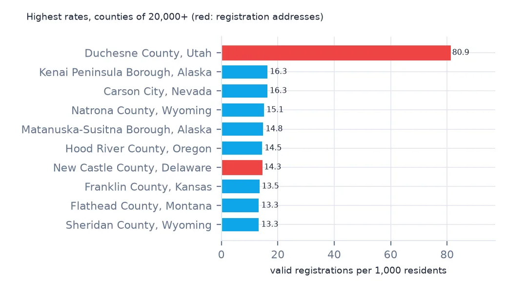
49013 Duchesne County Utah 1688.0 80.9
02122 Kenai Peninsula Borough Alaska 1012.0 16.3
32510 Carson City Nevada 954.0 16.3
56025 Natrona County Wyoming 1218.0 15.1
02170 Matanuska-Susitna Borough Alaska 1758.0 14.8
41027 Hood River County Oregon 343.0 14.5
10003 New Castle County Delaware 8401.0 14.3
20059 Franklin County Kansas 355.0 13.5
Duchesne County, UT: {'NORTH SALT LAKE': 1648, 'ROOSEVELT': 13} {'corporation': 1550, 'LLC': 91}
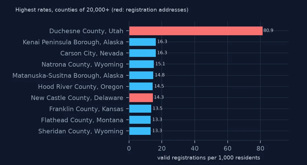
Duchesne County in eastern Utah tops the list at 80.9 aircraft per 1,000 residents, five times the next county. Its 1,688 aircraft are almost all corporation-owned, with a mailing city of North Salt Lake, which is not in Duchesne County at all: an address of convenience with a county code that does not even match it. New Castle County, Delaware, is in the list for the same kind of reason. Each of the others needs the same check of owner type and mailing city before it is read as a local fleet.
2. Individuals only
ind = us[us["TYPE REGISTRANT"] == "1"].GEOID.value_counts()
c["individual_per_1000"] = ind.reindex(c.index).fillna(0) / c.POPESTIMATE2025 * 1000
print(c[c.POPESTIMATE2025 >= 20_000].nlargest(8, "individual_per_1000")[["CTYNAME", "STNAME", "individual_per_1000"]].round(1).to_string())
print(f"rank correlation, all owners against individuals (20,000+ residents): "
      f"{c[c.POPESTIMATE2025 >= 20_000][['per_1000', 'individual_per_1000']].corr(method='spearman').iloc[0, 1]:.2f}")
CTYNAME STNAME individual_per_1000
GEOID
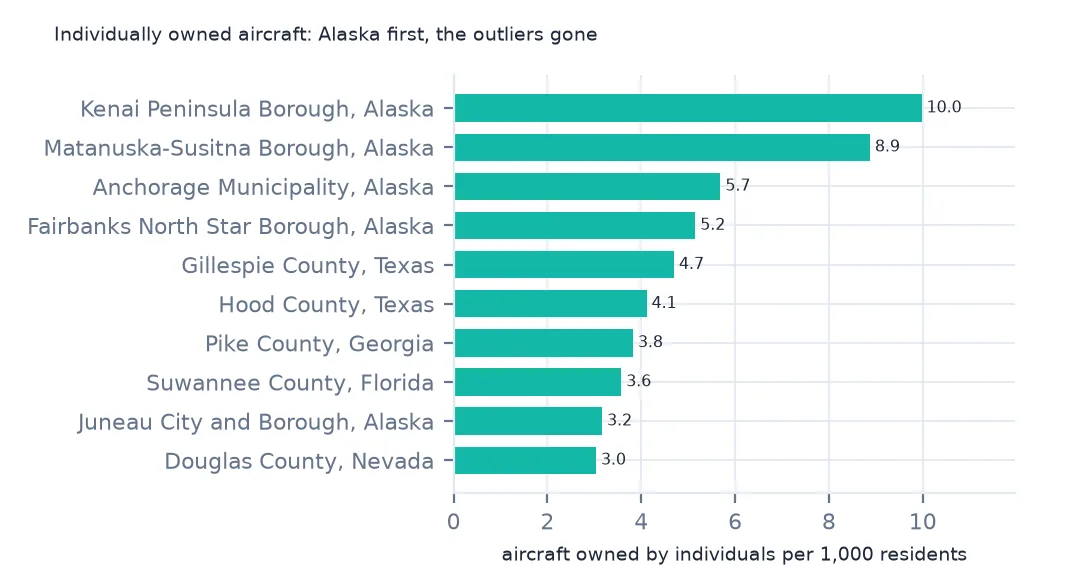
02122 Kenai Peninsula Borough Alaska 10.0
02170 Matanuska-Susitna Borough Alaska 8.9
02020 Anchorage Municipality Alaska 5.7
02090 Fairbanks North Star Borough Alaska 5.2
48171 Gillespie County Texas 4.7
48221 Hood County Texas 4.1
13231 Pike County Georgia 3.8
12121 Suwannee County Florida 3.6
rank correlation, all owners against individuals (20,000+ residents): 0.86
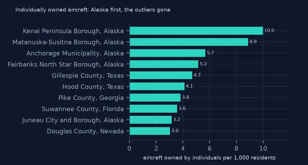
Counting only aircraft registered to individuals, who use their home address, the top of the list is Alaska: the Kenai Peninsula and Matanuska-Susitna boroughs at 10.0 and 8.9 per 1,000, then Anchorage and Fairbanks. Gillespie and Hood counties in Texas and Pike County, Georgia, follow. The two rankings still correlate at 0.86, but the outliers are gone.
3. The rows that did not join
lost = us[~us.GEOID.isin(c.index)]
print(f"valid US registrations with no county: {len(lost):,} ({len(lost) / len(us):.1%}); by state: {lost.STATE.value_counts().head(4).to_dict()}")
valid US registrations with no county: 3,586 (1.2%); by state: {'FL': 1606, 'CT': 1590, 'AK': 336, 'VA': 13}
3,586 valid US registrations, 1.2%, have a county code that is not in the 2024 county list: Florida 1,606, Connecticut 1,590 and Alaska 336. They are codes that no longer exist, and the fix page puts them back.
States and the map
The data used on this page
The FAA's Releasable Aircraft Database, public domain, downloaded on 16 October 2026 and saved on this site, because the FAA replaces it every day. The saved copy leaves out the owners' names and street addresses and keeps five-digit ZIP codes; every other column is as published. With it come the Census Bureau's Vintage 2025 county population estimates, 2024 county boundaries and 2024 ZCTA gazetteer.
from pathlib import Path
import zipfile

import geopandas as gpd
import numpy as np
import pandas as pd
import requests

Path("data").mkdir(exist_ok=True)
# FAA Releasable Aircraft Database, 16 October 2026: MASTER.txt without the NAME, STREET, STREET2 and OTHER NAMES
# columns and with five-digit ZIP codes (MASTER-no-names.txt), ACFTREF.txt and ENGINE.txt as published; Census
# Vintage 2025 county estimates, 2024 cartographic boundary counties and 2024 ZCTA gazetteer. Saved here unchanged
# otherwise, because the FAA replaces the file daily.
# Live: https://registry.faa.gov/database/ReleasableAircraft.zip (needs a browser User-Agent),
# https://www2.census.gov/geo/docs/maps-data/data/gazetteer/2024_Gazetteer/2024_Gaz_zcta_national.zip
ARCHIVE = "faa-aircraft-registry-2026-10-16.zip"
if not Path(f"data/{ARCHIVE}").exists():
    Path(f"data/{ARCHIVE}").write_bytes(requests.get(f"https://data.spatialworkflow.io/{ARCHIVE}", timeout=600).content)
Z = zipfile.ZipFile(f"data/{ARCHIVE}")


def faa(name):
    """One registry file: comma-separated, every field padded with spaces, a byte-order mark and a trailing comma."""
    d = pd.read_csv(Z.open(name), dtype=str, encoding="utf-8-sig", keep_default_na=False)
    d.columns = d.columns.str.strip()
    d = d.loc[:, [c for c in d.columns if c and not c.startswith("Unnamed")]]
    return d.apply(lambda c: c.str.strip())


reg = faa("MASTER-no-names.txt")
ref = faa("ACFTREF.txt")
TYPE_AIRCRAFT = {"1": "glider", "2": "balloon", "3": "blimp", "4": "fixed wing single engine", "5": "fixed wing multi engine",
                 "6": "rotorcraft", "7": "weight-shift", "8": "powered parachute", "9": "gyroplane", "H": "hybrid lift", "O": "other"}
REGISTRANT = {"1": "individual", "2": "partnership", "3": "corporation", "4": "co-owned", "5": "government", "7": "LLC",
              "8": "non-citizen corporation", "9": "non-citizen co-owned", "": "blank"}
Path("data/cb_2024_us_county_20m.zip").write_bytes(Z.read("cb_2024_us_county_20m.zip"))
counties = gpd.read_file("data/cb_2024_us_county_20m.zip")
STATEFP = counties.drop_duplicates("STUSPS").set_index("STUSPS").STATEFP
pop = pd.read_csv(Z.open("co-est2025-alldata.csv"), encoding="latin-1", dtype={"STATE": str, "COUNTY": str})
pop = pop[pop.SUMLEV == 50].assign(GEOID=lambda p: p.STATE + p.COUNTY)
print(f"FAA registry, 16 October 2026: {len(reg):,} aircraft, {len(ref):,} make-and-model codes")
FAA registry, 16 October 2026: 317,604 aircraft, 94,115 make-and-model codes
Example 1: by state
s = c.groupby("STNAME")[["aircraft", "POPESTIMATE2025"]].sum()
s["per_1000"] = s.aircraft / s.POPESTIMATE2025 * 1000
s = s.sort_values("per_1000")
print("highest:", ", ".join(f"{k} {v:.1f}" for k, v in s.per_1000.tail(5).iloc[::-1].items()))
print("lowest:", ", ".join(f"{k} {v:.2f}" for k, v in s.per_1000.head(4).items()))
highest: Alaska 11.8, Delaware 10.2, Wyoming 5.4, Montana 5.2, North Dakota 3.1
lowest: Connecticut 0.00, New Jersey 0.31, Rhode Island 0.32, New York 0.33
Alaska has 11.8 registered aircraft per 1,000 residents and Delaware 10.2, then Wyoming, Montana and North Dakota. Connecticut shows 0.00 only because none of its county codes join (they are the old counties); New Jersey, Rhode Island and New York have the fewest after it.
Example 2: the map, individual owners
low48 = counties[~counties.STUSPS.isin(["AK", "HI", "PR"])].to_crs(5070)
m = low48.merge(c[["individual_per_1000"]], left_on="GEOID", right_index=True, how="left")
m["cls"] = pd.cut(m.individual_per_1000, [0, 0.25, 0.5, 1, 2, 4, 100], right=False)
print(m.cls.value_counts(sort=False).to_string())
ax = m.plot(column="cls", cmap="Blues", legend=True, missing_kwds={"color": "lightgrey"}, figsize=(10, 6))
ax.set_axis_off()
cls
[0.0, 0.25) 605
[0.25, 0.5) 898
[0.5, 1.0) 893
[1.0, 2.0) 467
[2.0, 4.0) 189
[4.0, 100.0) 57
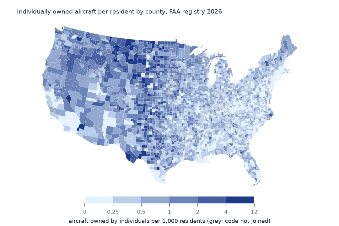
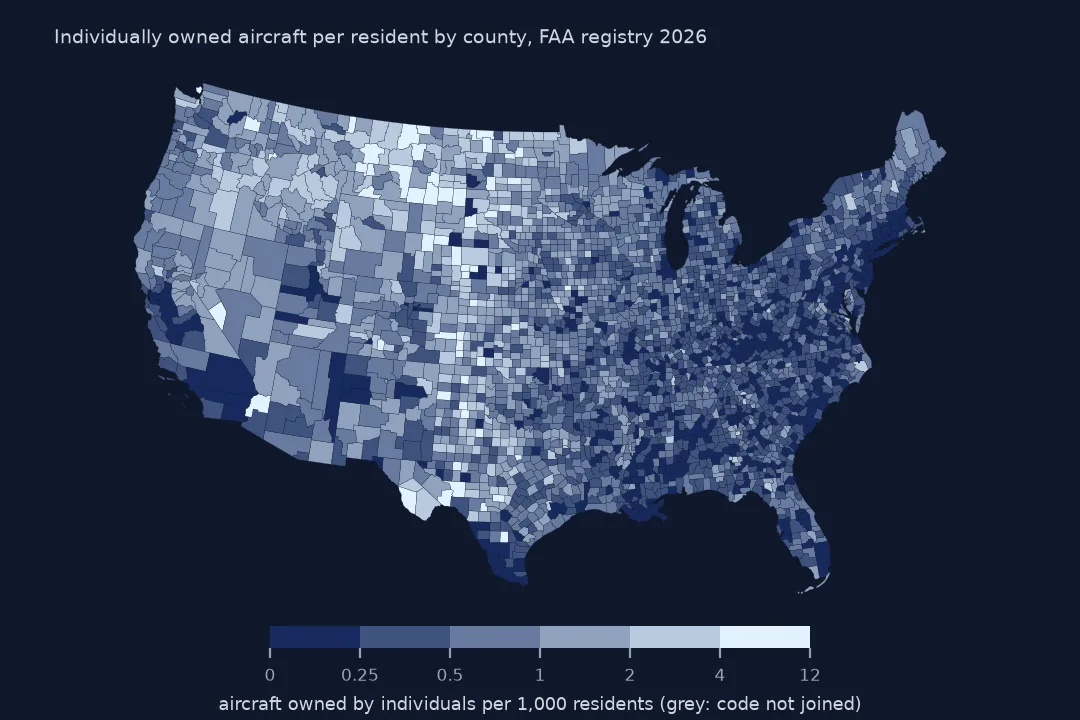
On the individual-owner map, 57 counties have 4 or more aircraft per 1,000 residents and 605 fewer than 0.25. The high counties run through the Mountain West, the northern Plains and rural Texas, and the low ones are the big cities and much of the Southeast.
Internal links
- Read the FAA registry — the
faa()reader and the columns - Registration addresses — why companies make a poor map of where aircraft are
- County codes that no longer exist — putting the unjoined rows back
- Fly-in communities by ZIP code — the same question at a finer scale