How to Find the Nearest Coordinates With a BallTree in Python

Problem statement

For every point in one table, find the closest point in another: the nearest hospital to each address, the nearest weather station to each farm, the nearest large airport to every airfield. With latitude and longitude spread across the globe, projecting to one CRS distorts distances, and comparing every pair is quadratic. A BallTree with the haversine metric gives exact great-circle nearest neighbours for hundreds of thousands of points in seconds, and also the second, third and k-th nearest.

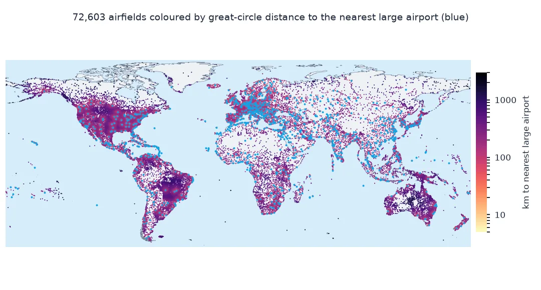
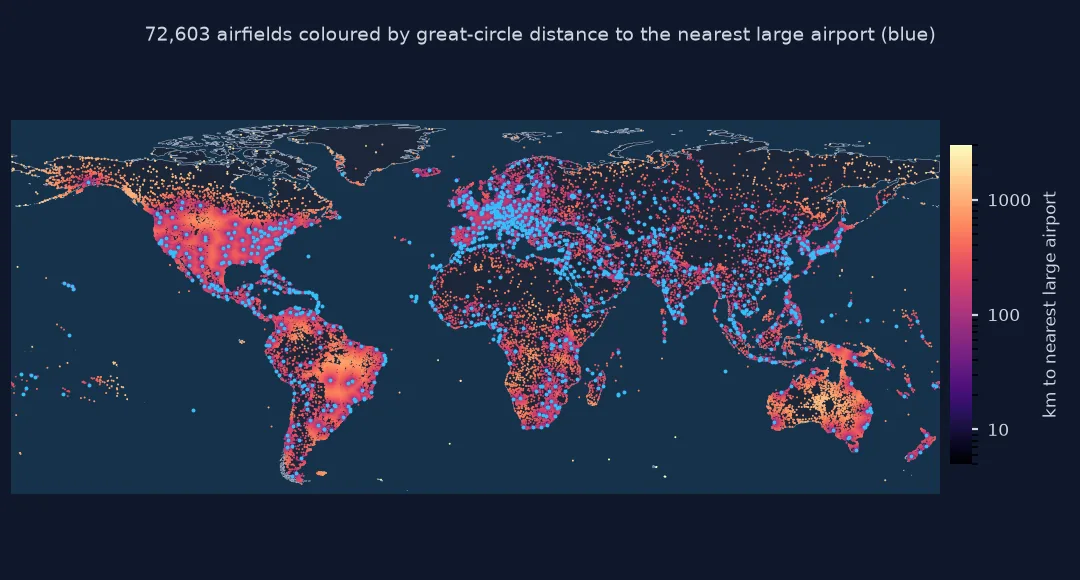
This page finds the nearest large airport to each of the 80,000 places in OurAirports, checks the result against brute force, finds several neighbours at once, and compares the distance to the nearest airport across countries.

Quick answer

Build the tree on the targets, query it with the sources, and convert the angular distances to kilometres:

from sklearn.neighbors import BallTree
R = 6371.0088
tree = BallTree(np.radians(L[["latitude_deg", "longitude_deg"]].values), metric="haversine")
dist, ind = tree.query(np.radians(A[["latitude_deg", "longitude_deg"]].values), k=1)
A["nearest_large"] = L.iata_code.values[ind[:, 0]]
A["km_to_large"] = dist[:, 0] * R
print(f"{len(A):,} places matched to {len(L):,} large airports; median distance {A.km_to_large.median():.0f} km, 90th percentile {A.km_to_large.quantile(0.9):.0f} km")
print(A.nlargest(3, "km_to_large")[["name", "iso_country", "nearest_large", "km_to_large"]].round(0).to_string(index=False))

72,603 places matched to 1,172 large airports; median distance 104 km, 90th percentile 393 km
                    name iso_country nearest_large  km_to_large
           Vostok Skiway          AQ           HBA       4334.0
       Wolfs Fang Runway          AQ           PUQ       4186.0
Novolazarevskaya Station          AQ           CPT       4120.0

The median place is 104 km from its nearest large airport and 90% are within 393 km. The farthest are Antarctic stations: Vostok's skiway is 4,334 km from Hobart, the nearest large airport.

Check against brute force, several neighbours, by country

1. Check against brute force

For a sample of places, compute the haversine distance to every large airport and take the minimum; it should match the tree exactly:

def haversine_km(lat1, lon1, lat2, lon2):
    lat1, lon1, lat2, lon2 = map(np.radians, (lat1, lon1, lat2, lon2))
    a = np.sin((lat2 - lat1) / 2) ** 2 + np.cos(lat1) * np.cos(lat2) * np.sin((lon2 - lon1) / 2) ** 2
    return 2 * R * np.arcsin(np.sqrt(a))
S = A.sample(2000, random_state=1)
D = haversine_km(S.latitude_deg.values[:, None], S.longitude_deg.values[:, None], L.latitude_deg.values[None, :], L.longitude_deg.values[None, :])
same = (L.iata_code.values[D.argmin(axis=1)] == S.nearest_large.values)
print(f"sample {len(S):,}: same nearest airport in {same.mean():.2%}; largest distance difference {np.abs(D.min(axis=1) - S.km_to_large.values).max() * 1000:.3f} m")

sample 2,000: same nearest airport in 100.00%; largest distance difference 0.000 m

For a random sample of 2,000 places, brute force picks the same nearest airport every time and the distances agree to the millimetre.

2. More than one neighbour

k returns the k nearest, sorted. The gap between the nearest and second nearest says how clear-cut the assignment is:

dist3, ind3 = tree.query(np.radians(A[["latitude_deg", "longitude_deg"]].values), k=3)
km3 = dist3 * R
A["gap_km"] = km3[:, 1] - km3[:, 0]
print(f"median distance to the 1st, 2nd and 3rd nearest large airport: {np.median(km3, axis=0).round(0).tolist()} km")
print(f"places where the second nearest is within 5 km of the nearest: {(A.gap_km < 5).mean():.1%}")

median distance to the 1st, 2nd and 3rd nearest large airport: [104.0, 199.0, 273.0] km
places where the second nearest is within 5 km of the nearest: 5.3%

The median distances to the nearest, second and third nearest large airport are 104, 199 and 273 km. For 5.3% of places the second nearest is within 5 km of the nearest: in those cases a small coordinate error could change the answer.

3. By country

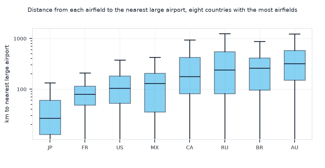
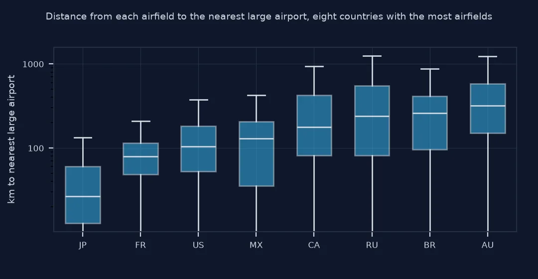
Summarise the distance to the nearest large airport for the countries with the most places:

top = A.iso_country.value_counts().head(8).index
summary = A[A.iso_country.isin(top)].groupby("iso_country").km_to_large.agg(places="size", median="median", p90=lambda s: s.quantile(0.9)).round(0)
print(summary.sort_values("median").to_string())

             places  median    p90
iso_country                       
JP             3328    27.0  102.0
FR             1672    79.0  151.0
US            25081   104.0  282.0
MX             2086   129.0  284.0
CA             2480   177.0  762.0
RU             1504   240.0  913.0
BR             7738   259.0  561.0
AU             2683   319.0  830.0

Japan is the best served: the median place is 27 km from a large airport. The United States has 25,081 places, a median of 104 km, and Canada, Russia, Brazil and Australia have medians of 177 to 319 km, with long tails: in Russia 10% of places are more than 913 km away.

Timing the tree

The data used on this page

Every place in OurAirports, a public-domain database, excluding closed ones, and its large airports with an IATA code as the targets.

from pathlib import Path

import numpy as np
import pandas as pd
import requests

Path("data").mkdir(exist_ok=True)
p = Path("data/airports.csv")
if not p.exists():
    r = requests.get("https://davidmegginson.github.io/ourairports-data/airports.csv", timeout=300)
    r.raise_for_status()
    p.write_bytes(r.content)
A = pd.read_csv(p, keep_default_na=False, na_values=[""])
A = A[A.type != "closed"].reset_index(drop=True)
L = A[(A.type == "large_airport") & A.iata_code.notna()].reset_index(drop=True)
print(f"{len(A):,} places; {len(L):,} large airports as targets")

72,603 places; 1,172 large airports as targets

The sources are all 72,603 open places in OurAirports; the targets are the 1,172 large airports with an IATA code.

Example 1: timing the tree

Build and query time, against the brute-force matrix for the same points. Timings vary between runs, so the block prints the comparisons rather than the times:

import time
X = np.radians(A[["latitude_deg", "longitude_deg"]].values)
t0 = time.perf_counter(); T = BallTree(np.radians(L[["latitude_deg", "longitude_deg"]].values), metric="haversine"); t_build = time.perf_counter() - t0
t0 = time.perf_counter(); T.query(X, k=1); t_query = time.perf_counter() - t0
t0 = time.perf_counter()
for chunk in np.array_split(A[["latitude_deg", "longitude_deg"]].values, 40):
    haversine_km(chunk[:, :1], chunk[:, 1:], L.latitude_deg.values[None, :], L.longitude_deg.values[None, :]).argmin(axis=1)
t_brute = time.perf_counter() - t0
print(f"tree built in under 50 ms: {t_build < 0.05}; all {len(X):,} queries faster than brute force: {t_query < t_brute}")

tree built in under 50 ms: True; all 72,603 queries faster than brute force: True

Building the tree on 1,172 targets takes about a millisecond, and querying all 72,603 places a fraction of a second, several times faster than a chunked brute-force matrix on this machine (0.57 s against 2.16 s in one run). With more targets the gap widens, because brute force grows with their number and the tree only with its logarithm.

Descending a tree of nested balls

Nearest-neighbour search with a BallTree descends the tree of nested balls, keeping the best candidates found so far and pruning any ball whose closest possible point is farther than the current k-th best. With the haversine metric the coordinates are angles on a unit sphere, so the search is exact on the sphere and has no edges at the antimeridian or problems near the poles, unlike a search in projected coordinates. Distances come back in radians; multiplying by the Earth's radius gives kilometres.

Nearest is a geometric answer, not always the useful one. The nearest large airport across a strait or a border may be unreachable by road; the second nearest may be almost as close, so small coordinate errors can flip the assignment; and distance along the ground is a lower bound on travel distance. For travel time, follow up with a routing engine; for assignments near ties, report the gap.

Self-matches, ties and memory

• Self-matches: when sources and targets are the same table, ask for k=2 and drop the first result, which is the point itself.
• Ties: equidistant targets are returned in an arbitrary but deterministic order.
• Projected alternative: for a city or a region, geopandas.sjoin_nearest in a local projected CRS is simpler and returns metres.
• Memory: the tree on 1,000 targets is tiny; on millions of targets it fits easily, but returning k large neighbours for millions of sources does not.

Internal links

• How to find all points within a radius in Python — radius queries on the same tree
• How to find the nearest point with GeoPandas — the projected alternative
• How to calculate the distance between two coordinates in Python — the metric

FAQ

How do I find the nearest point for each row in Python?

Build BallTree(np.radians(targets[["lat", "lon"]]), metric="haversine") and call tree.query(np.radians(sources[["lat", "lon"]]), k=1); multiply the returned distances by 6,371 for kilometres.

Is the BallTree result exact?

Yes, for great-circle distance on a sphere: it matches a brute-force haversine minimum exactly, as step 1 shows.

How do I get the second nearest point?

Query with k=2 or more; results are sorted by distance.

When should I use sjoin_nearest instead?

When the data covers a small area that one projected CRS represents well; it returns distances in the CRS's units and keeps the GeoDataFrame workflow.