How to Find All Points Within a Radius in Python

Problem statement

"Every store within 5 km of each customer", "all airports within 100 km of this point", "how many sensors within 50 km": radius queries are among the most common spatial questions, and with latitude-longitude data they need a great-circle distance, not a buffer in degrees. A brute-force loop over all pairs is fine for hundreds of points and hopeless for hundreds of thousands. A spatial index such as scikit-learn's BallTree with the haversine metric answers the same queries in milliseconds and returns exact great-circle results.

This page runs radius queries on the 80,000 places in OurAirports: all airfields within 100 km of a point by brute force and with a BallTree, counts of neighbours within a radius for every large airport at once, a check that both methods agree exactly, and timings that show where the index pays off.

Quick answer

Build a BallTree on coordinates in radians with the haversine metric, and give the radius in radians (kilometres divided by the Earth's radius):

from sklearn.neighbors import BallTree
R = 6371.0088
tree = BallTree(np.radians(A[["latitude_deg", "longitude_deg"]].values), metric="haversine")
lhr = A[A.iata_code == "LHR"].iloc[0]
idx, dist = tree.query_radius(np.radians([[lhr.latitude_deg, lhr.longitude_deg]]), r=100 / R, return_distance=True, sort_results=True)
near = A.iloc[idx[0]].assign(km=dist[0] * R)
print(f"places within 100 km of LHR: {len(near):,}; of which large or medium airports: {near.type.isin(['large_airport', 'medium_airport']).sum()}")
print(near[near.type.isin(["large_airport", "medium_airport"])][["ident", "name", "km"]].head(6).round(1).to_string(index=False))

places within 100 km of LHR: 315; of which large or medium airports: 21
ident                       name   km
 EGLL    London Heathrow Airport  0.0
 EGWU               RAF Northolt  9.6
 EGLF        Farnborough Airport 30.9
 EGLK         Blackbushe Airport 31.5
 EGLC        London City Airport 35.9
 EGKB London Biggin Hill Airport 37.5

315 places lie within 100 km of Heathrow, 21 of them large or medium airports. Results come sorted by distance: RAF Northolt at 9.6 km, Farnborough at 30.9 km, London City at 35.9 km.

Brute force, many queries, when an index pays off

1. The brute-force answer

Compute the haversine distance from the point to every row and filter. It is the reference the index must match:

def haversine_km(lat1, lon1, lat2, lon2):
    lat1, lon1, lat2, lon2 = map(np.radians, (lat1, lon1, lat2, lon2))
    a = np.sin((lat2 - lat1) / 2) ** 2 + np.cos(lat1) * np.cos(lat2) * np.sin((lon2 - lon1) / 2) ** 2
    return 2 * R * np.arcsin(np.sqrt(a))
d = haversine_km(lhr.latitude_deg, lhr.longitude_deg, A.latitude_deg.values, A.longitude_deg.values)
brute = set(np.where(d <= 100)[0])
print(f"brute force: {len(brute):,} places; same set as the BallTree: {brute == set(idx[0])}")

brute force: 315 places; same set as the BallTree: True

The brute-force filter finds the same 315 places: the BallTree is exact, not an approximation.

2. Many queries at once

Count the places within 50 km of every large airport in one call with count_only=True:

L = A[A.type == "large_airport"]
counts = tree.query_radius(np.radians(L[["latitude_deg", "longitude_deg"]].values), r=50 / R, count_only=True) - 1
L = L.assign(within_50km=counts)
print(f"large airports: {len(L):,}; median places within 50 km: {np.median(counts):.0f}")
print(L.nlargest(5, "within_50km")[["iata_code", "municipality", "within_50km"]].to_string(index=False))

large airports: 1,175; median places within 50 km: 5
iata_code municipality  within_50km
      HND        Tokyo          909
      GMP        Seoul          633
      ITM        Osaka          580
      UKB         Kobe          568
      KIX        Osaka          552

Counting is a single call for all 1,175 large airports. The median large airport has 5 other places within 50 km, but Tokyo Haneda has 909, of which 897 are heliports, and Seoul Gimpo 633: in Japan and Korea heliports on buildings and hospitals crowd the cities.

3. When the index pays off

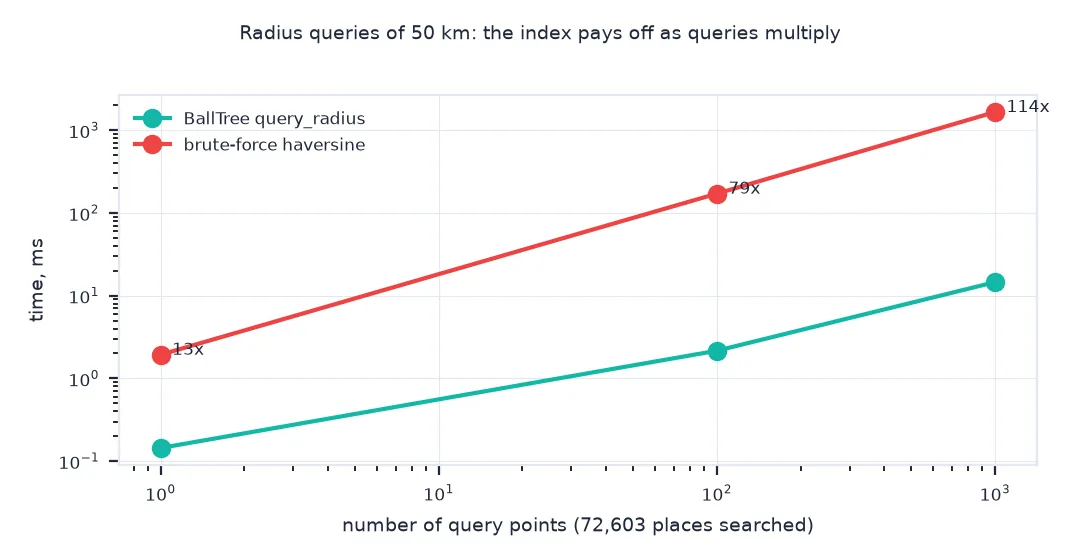
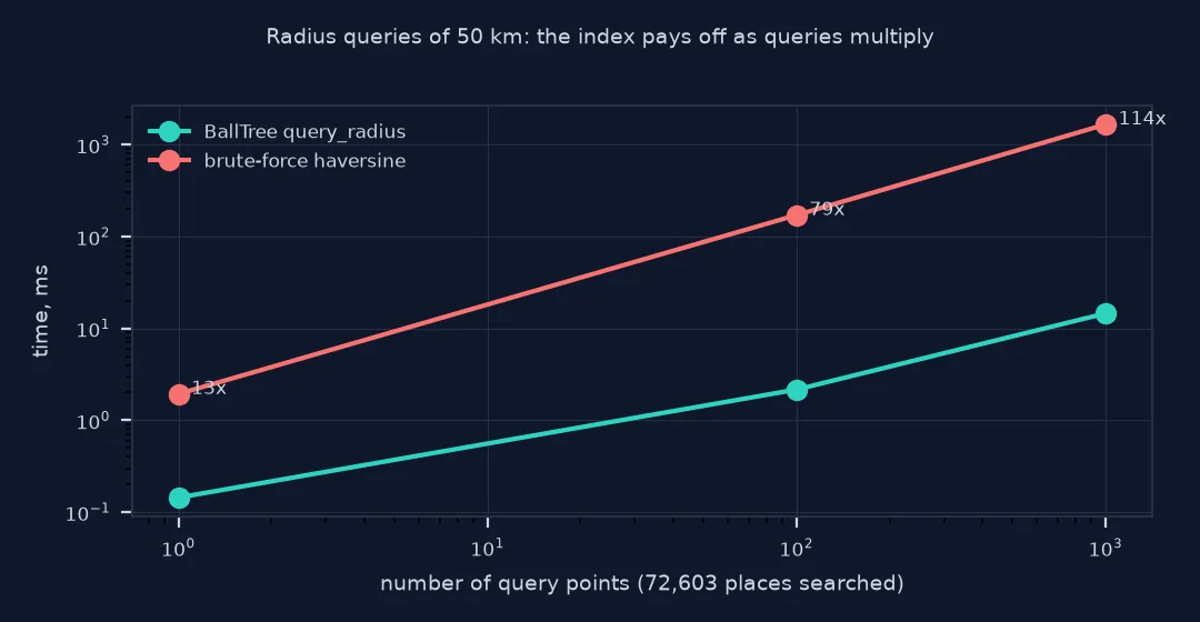
Time both approaches for growing numbers of query points. Timings change from run to run, so the block prints whether the speed-up clears a threshold, and the chart below shows one measured run:

import time
rows = []
for nq in (1, 100, 1000):
    Q = A.sample(nq, random_state=0)[["latitude_deg", "longitude_deg"]].values
    t0 = time.perf_counter(); tree.query_radius(np.radians(Q), r=50 / R, count_only=True); t_tree = time.perf_counter() - t0
    t0 = time.perf_counter(); [(haversine_km(q[0], q[1], A.latitude_deg.values, A.longitude_deg.values) <= 50).sum() for q in Q]; t_brute = time.perf_counter() - t0
    rows.append((nq, t_tree, t_brute))
for (nq, a_, b_), need in zip(rows, (2, 20, 50)):            # timings vary between runs; the thresholds do not
    print(f"{nq:>5} queries: BallTree more than {need}x faster than brute force: {b_ / a_ > need}")

    1 queries: BallTree more than 2x faster than brute force: True
  100 queries: BallTree more than 20x faster than brute force: True
 1000 queries: BallTree more than 50x faster than brute force: True

For one query the tree is roughly ten times faster than a vectorised pass over 72,603 rows; for 1,000 queries it is about a hundred times faster, a few hundredths of a second against nearly two seconds on this machine.

A radius in degrees, done wrong

The data used on this page

Every place in OurAirports, a public-domain database of airports, airfields, heliports and seaplane bases, excluding closed ones. The BallTree is scikit-learn's sklearn.neighbors.BallTree.

from pathlib import Path

import numpy as np
import pandas as pd
import requests

Path("data").mkdir(exist_ok=True)
p = Path("data/airports.csv")
if not p.exists():
    r = requests.get("https://davidmegginson.github.io/ourairports-data/airports.csv", timeout=300)
    r.raise_for_status()
    p.write_bytes(r.content)
A = pd.read_csv(p, keep_default_na=False, na_values=[""])
A = A[A.type != "closed"].reset_index(drop=True)
print(f"{len(A):,} places; types {A.type.value_counts().to_dict()}")

72,603 places; types {'small_airport': 42766, 'heliport': 23220, 'medium_airport': 4106, 'seaplane_base': 1273, 'large_airport': 1175, 'balloonport': 63}

Without closed sites, OurAirports lists 72,603 places: 42,766 small airports, 23,220 heliports, 4,106 medium and 1,175 large airports, 1,273 seaplane bases and 63 balloonports.

Example 1: the radius in degrees, done wrong

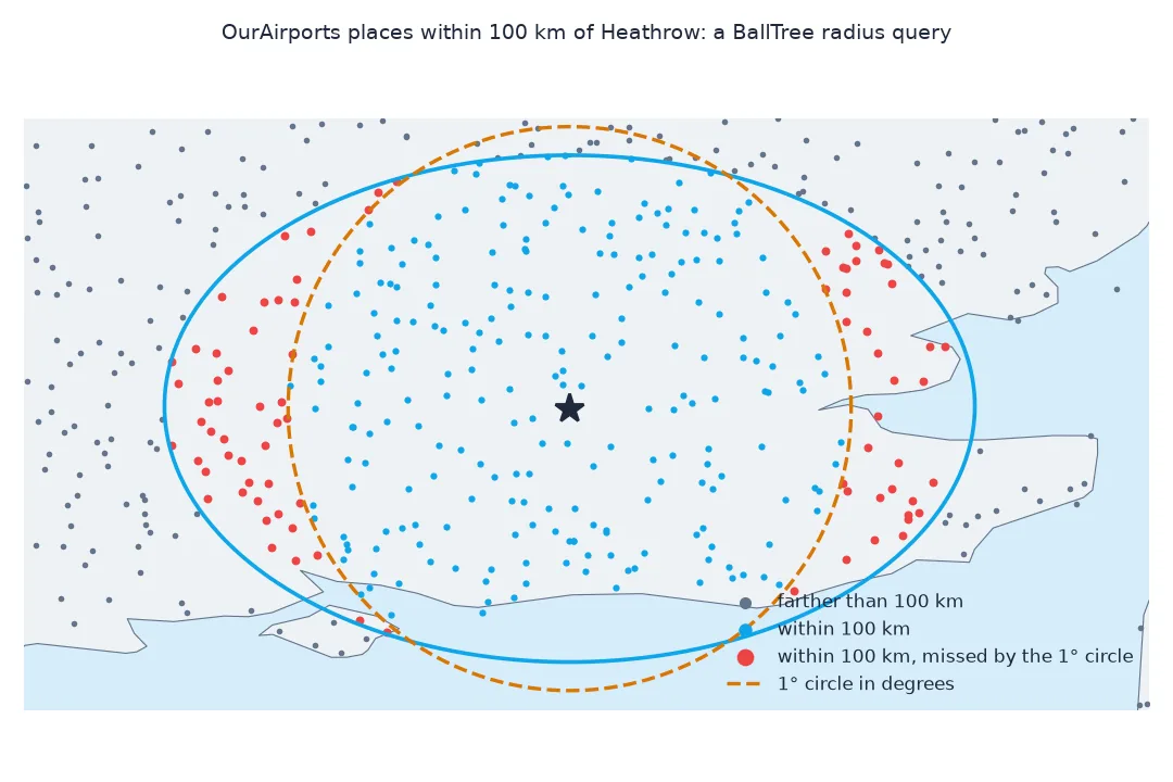
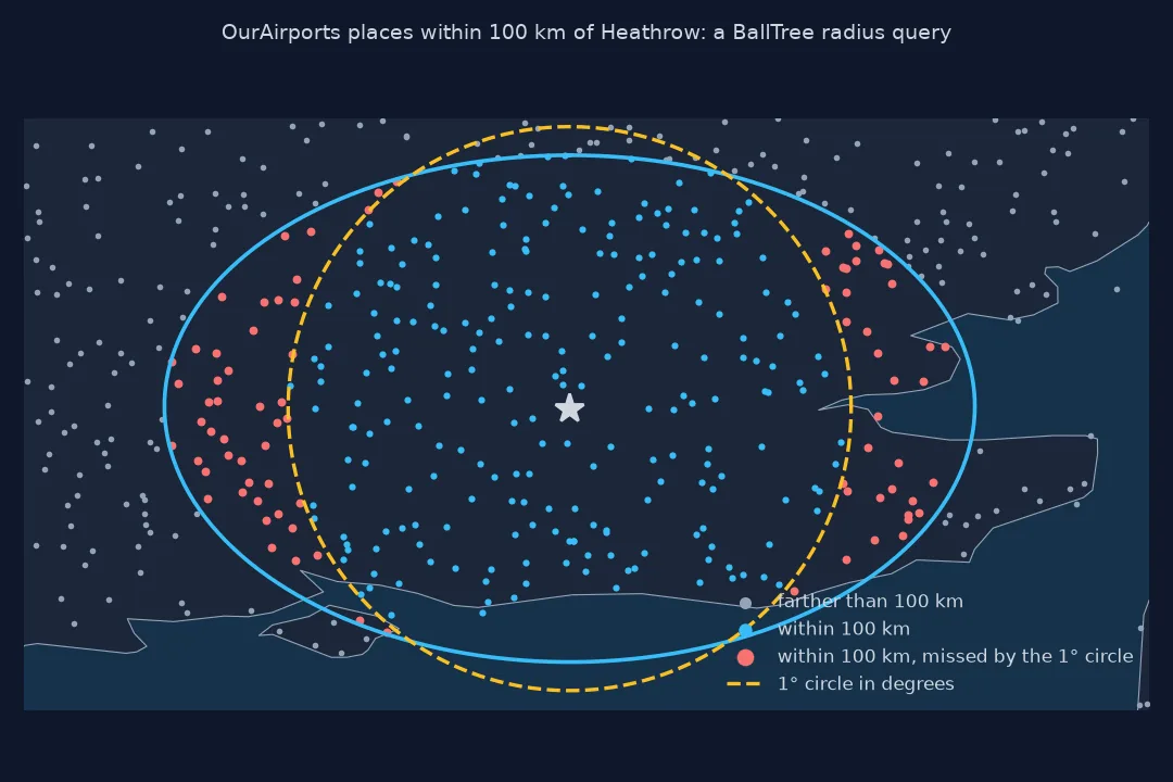
A common shortcut filters by a box or circle in degrees. Compare a 1° "radius" with the true 100 km result at Heathrow:

in_deg = np.hypot(A.latitude_deg - lhr.latitude_deg, A.longitude_deg - lhr.longitude_deg) <= 1
true = d <= 100
print(f"1° circle: {in_deg.sum():,} places; true 100 km circle: {true.sum():,}")
print(f"in the degree circle but farther than 100 km: {(in_deg & ~true).sum()}; within 100 km but outside the degree circle: {(true & ~in_deg).sum()}")
print(f"farthest place caught by the degree circle: {d[in_deg].max():.0f} km")

1° circle: 244 places; true 100 km circle: 315
in the degree circle but farther than 100 km: 11; within 100 km but outside the degree circle: 82
farthest place caught by the degree circle: 107 km

A circle of 1° around Heathrow catches 244 places against 315 within the true 100 km: it reaches 111 km north and south but only 69 km east and west at this latitude. It misses 82 places that are within 100 km and includes 11 that are not, the farthest 107 km away.

How a BallTree skips whole groups

A BallTree partitions points into nested hyperspheres, balls, so a query can skip whole groups that are too far away to contain any match. With the haversine metric, scikit-learn treats the coordinates as latitude and longitude in radians on a unit sphere, so radii and returned distances are angles: multiply by the Earth's radius for kilometres. The results are exact great-circle distances on that sphere, identical to a brute-force haversine filter, which step 1 confirms.

The cost model explains when to use it. Building the tree takes a fraction of a second for 80,000 points; each query then touches only a small part of the data. A single query is barely faster than a vectorised brute-force pass, because NumPy is fast; for thousands of queries the index wins by orders of magnitude. For radius joins between two GeoDataFrames, project to a suitable CRS and use sjoin_nearest or sjoin with buffers, or keep the BallTree for latitude-longitude data spread across the globe, where no single projection is accurate.

Column order, spheres and the KD-tree alternative

• Order of columns: the haversine metric expects latitude first, then longitude, in radians.
• Sphere, not ellipsoid: distances can be up to about 0.5% off; points right at the edge of a radius may flip.
• Antimeridian and poles: the haversine BallTree has no seam; boxes in degrees do.
• KD-tree alternative: convert to 3D unit vectors and use scipy.spatial.cKDTree with chord distances, as on the plate boundaries page.

Internal links

• How to find the nearest coordinates with a BallTree in Python — k-nearest queries
• How to calculate the distance between two coordinates in Python — the distance used here
• Fixing buffers drawn in degrees instead of kilometres — the degree trap

FAQ

How do I find all points within a radius of a coordinate in Python?

Build BallTree(np.radians(latlon), metric="haversine") and call query_radius(np.radians([[lat, lon]]), r=km / 6371.0088).

Why do I divide the radius by 6,371?

The haversine BallTree works on the unit sphere in radians; dividing kilometres by the Earth's radius converts the radius to an angle.

Is a BallTree faster than computing all distances?

For many queries, yes, by orders of magnitude; for a single query a vectorised NumPy pass is nearly as fast.

Can I use a radius in degrees instead?

Only as a rough pre-filter: a degree of longitude is much shorter than a degree of latitude away from the equator.