Differential privacy for spatial counts explained #

Problem statement #

Suppression and masking both answer the question "is this release safe?". Differential privacy answers a harder one: "is this release safe given everything else I have published and will publish?" It does that by adding calibrated random noise and keeping a budget, so that the guarantee degrades in a known way instead of silently.

The mechanics are simple enough to write in three lines. What is hard is the accounting:

• Noise is calibrated to sensitivity — how much one person can change the answer — not to the size of the count.
• Every query spends ε from a fixed budget, and the budget covers everything, including the query you ran to choose the cell size.
• The noise is largest, in relative terms, exactly where the counts are smallest, which is where spatial data is most interesting.

This guide covers what ε means for a map, how the Laplace mechanism behaves on real cell counts, and when the answer is to use aggregation instead.

Quick answer #

Add Laplace noise with scale 1/ε to each cell count, then post-process:

import numpy as np

rng = np.random.default_rng(7)

def private_counts(counts, epsilon, sensitivity=1):
    noisy = counts + rng.laplace(0, sensitivity / epsilon, len(counts))
    return np.maximum(np.round(noisy), 0)          # post-processing is free

released = private_counts(cell_counts.values, epsilon=1.0)

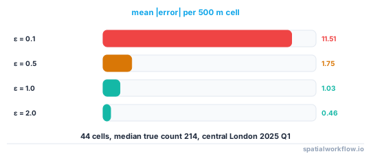
On 44 cells of 500 m London crime counts, ε=1.0 gave a mean absolute error of 1.03 crimes and a 95th percentile of 2.96 — negligible against a median cell count of 214. At ε=0.1 the same cells had a mean error of 11.51 and two cells went negative.

Step-by-step solution #

1. Define the unit of privacy #

ε protects a neighbouring dataset: one where a single unit is added or removed. That unit must be stated. "One event" is easy to implement and weak, because one person can generate fifty events. "One person" is what people assume you mean, and it makes the sensitivity of a count equal to the maximum number of events one person can contribute.

2. Compute the sensitivity honestly #

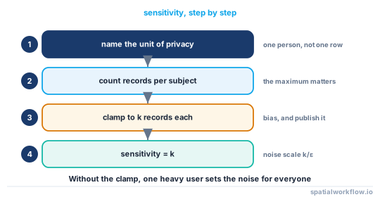
For a count where each person contributes at most one record, sensitivity is 1. If a person can appear in several cells — a trajectory, a set of repeat visits — the sensitivity is the maximum number of cells one person can affect, and the noise grows with it. Clamping contributions (at most k records per person) is the standard fix, and the clamp is itself a design decision to publish.

3. Pick ε, and be honest that it is a policy choice #

There is no technical value of ε. Published deployments range from 0.1 to 10 or more; the US Census used a total budget in the tens across the whole 2020 product. What ε does is bound how much the odds of any inference about one person can shift: a factor of e^ε. At ε=1 that is 2.7×, at ε=0.1 it is 1.1×.

4. Apply the mechanism to the counts, not to the points #

Noising coordinates is a different and much harder problem (geo-indistinguishability). For maps, the standard construction is: aggregate to cells, add Laplace noise to each cell count, publish. The aggregation is what makes sensitivity small.

5. Post-process freely #

Anything you do to a differentially private output without touching the raw data is still differentially private. Clamping negatives to zero, rounding to integers, smoothing, and enforcing that a set of cells sums to a published total are all allowed and all improve usability.

6. Keep the budget #

Every published statistic derived from the raw data spends ε. Two maps at ε=1 are one release at ε=2. Choosing a cell size by looking at the data spends budget too. Write the budget down before you start, and treat it as a resource that does not refill.

7. Check what the noise did to small cells #

At ε=0.1 on the London cells, two of 44 cells went negative and two cells with a true count above zero were released as zero. That is the mechanism working as designed, and it is why differential privacy is a poor fit for maps whose interesting features are small counts.

Code examples #

Example 1 — the mechanism, and what ε costs #

import numpy as np

rng = np.random.default_rng(7)
counts = cell_counts.values          # 44 cells, 500 m, central London, 2025 Q1

print(f"{'eps':>5} {'mean |err|':>10} {'p95 |err|':>9} {'negatives':>10} {'true>0 -> 0':>12}")
for eps in (0.1, 0.5, 1.0, 2.0):
    noisy = counts + rng.laplace(0, 1 / eps, len(counts))
    err = np.abs(noisy - counts)
    clipped = np.maximum(np.round(noisy), 0)
    print(f"{eps:5.1f} {err.mean():10.2f} {np.percentile(err, 95):9.2f} "
          f"{int((noisy < 0).sum()):10,} {int(((counts > 0) & (clipped == 0)).sum()):12,}")

  eps mean |err| p95 |err|  negatives  true>0 -> 0
  0.1      11.51     44.42          2            2
  0.5       1.75      4.39          0            0
  1.0       1.03      2.96          0            0
  2.0       0.46      1.26          0            0

Example 2 — sensitivity when one person contributes many records #

def clamp_contributions(df, subject_col, k):
    """Keep at most k records per subject so sensitivity is bounded by k."""
    return df.groupby(subject_col, group_keys=False).head(k)

k = 3
clamped = clamp_contributions(visits, "patient_id", k)
print(f"kept {len(clamped):,} of {len(visits):,} records ({len(clamped)/len(visits):.1%})")

noisy = clamped.groupby("cell").size().reindex(all_cells, fill_value=0).values \
        + rng.laplace(0, k / 1.0, len(all_cells))     # sensitivity k, epsilon 1

Without the clamp, one frequent visitor sets the sensitivity for the whole release.

Example 3 — post-processing to a consistent, usable map #

noisy = np.maximum(np.round(counts + rng.laplace(0, 1.0, len(counts))), 0)

# enforce a published total (still differentially private: no raw data is touched)
target = noisy.sum()
scaled = np.round(noisy * (target / max(noisy.sum(), 1)))

print(f"cells: {len(noisy)}, zeros after clamping: {(noisy == 0).sum()}, "
      f"total drift vs truth: {noisy.sum() - counts.sum():+.0f}")

cells: 44, zeros after clamping: 0, total drift vs truth: -7

A seven-crime drift across 19,619 records is invisible in any use of the map, which is what ε=1 buys on counts this size.

Explanation #

Why noise rather than suppression #

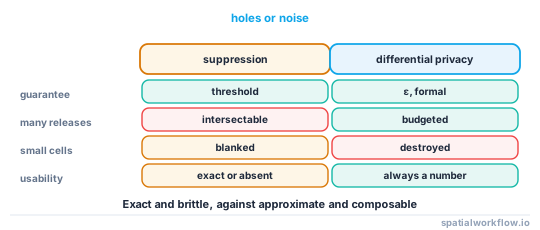
Suppression makes a binary promise about one release and composes badly: two suppression patterns over the same population can be intersected. Differential privacy makes a continuous promise that composes by addition — run two ε=1 queries and you have spent ε=2, and you know it. For a product published monthly for years, that accounting is the whole point.

Why ε has no natural value #

ε bounds the multiplicative change in the probability of any output when one person's data changes. Translating that into "acceptable" requires knowing the harm, the attacker's prior and the number of releases. Treat it as a published policy parameter, like a suppression threshold, and expose it in the metadata.

Why it fits counts and not points #

The Laplace mechanism needs bounded sensitivity. A count of people in a cell changes by at most one when one person is added, so sensitivity is 1 regardless of how many people there are. A coordinate has no such bound: moving one person can move a centroid arbitrarily far. Point-level differential privacy exists (geo-indistinguishability, which scales noise to a radius), but it is a different guarantee and a different budget.

Why the small cells lose #

Laplace noise has scale 1/ε whatever the count, so the relative error is the noise divided by the count. A cell of 3,533 crimes is untouched at ε=1; a cell of 2 is destroyed. If the purpose of the map is to find sparse events, differential privacy will not preserve them, and aggregation to larger units is the honest answer.

Edge cases or notes #

• ε is per release of the raw data, not per file. Re-running the mechanism spends more budget.
• Choosing parameters from the data spends budget. Picking a cell size by inspecting counts is a query.
• Negative counts are expected. Clamp them; do not resample, which breaks the guarantee.
• Zeros become ambiguous. A released zero may be a true zero or a noised small count — say so.
• The geometry is public. Differential privacy protects the counts, not the cell boundaries.
• Hierarchies need consistency post-processing. Cell counts that must sum to a region total need reconciling after noising.
• Small populations need larger ε to stay useful, which is the wrong direction. That tension is real and has no clean fix.
• Publish ε, the unit of privacy and the sensitivity. A release that says "differentially private" without them says nothing.

Internal links #

• How to add differentially private noise to spatial counts — the implementation with a budget ledger
• Aggregation and suppression rules explained — the alternative, and when it is better
• Suppressed cells can be recovered from the totals — the composition failure DP is designed to avoid
• Spatial k-anonymity explained — the guarantee DP replaces
• Geoprivacy explained: why coordinates are personal data — choosing between the three defences
• Counts, rates and densities explained — what noise does to a rate
• Small area rates explained — small denominators and noisy numerators
• How to smooth rates with empirical Bayes in Python — a different way to handle noisy small cells

FAQ #

What does ε actually promise? #

That the probability of any published output changes by at most a factor of e^ε when one person's data is added or removed. At ε=1 that is about 2.7×.

How much noise does ε=1 add to a map? #

Laplace noise with scale 1, so a mean absolute error of about one count per cell. On 500 m London crime cells with a median count of 214, the measured mean error was 1.03.

Can I add noise to coordinates instead of counts? #

That is geo-indistinguishability, a related but different guarantee whose noise is calibrated to a radius. The standard Laplace mechanism needs a bounded sensitivity, which counts have and coordinates do not.

What happens to small counts? #

They are swamped. At ε=0.1, two cells in the test went negative and two non-empty cells were released as zero. If sparse events are the point of the map, aggregate instead.

Is clamping negatives to zero allowed? #

Yes. Any post-processing that does not touch the raw data preserves the guarantee, including clamping, rounding and smoothing.

Do I still need suppression if I use differential privacy? #

No, and mixing them is usually a mistake: suppressing noisy cells reintroduces a data-dependent decision that is not covered by the budget.