
Geomasking methods explained: donut, random and adaptive
Problem statement
Geomasking moves each point somewhere it did not happen, far enough that an attacker cannot tell which address it came from and near enough that the analysis still works. Every method in the family is that one trade, parameterised differently, and the parameters decide both halves.
The three that matter in practice:
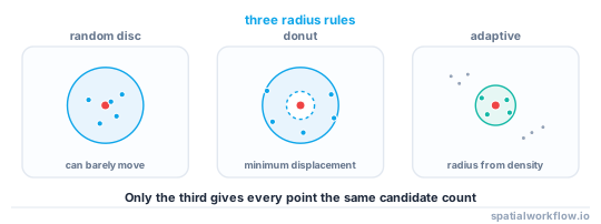
- Random perturbation — displace by a uniform draw inside a disc of radius R. Simple, and it leaves a fifth of points within 0.45R of the truth.
- Donut masking — the same, with an inner radius so no point can stay nearly where it was.
- Adaptive (density-based) masking — size each point's radius from how many candidate subjects surround it, so protection is equal instead of displacement being equal.
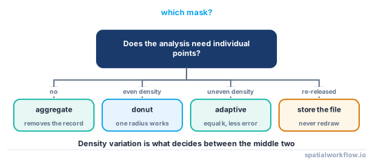
There is also aggregation to a unit, which is not masking at all and is usually the better answer. This guide covers what each method does to a real dataset — 3,109 OpenStreetMap address points in Brighton & Hove — and how to choose between them.
Quick answer
Donut-mask with a correctly drawn radius, then check displacement and validity:
import numpy as np

rng = np.random.default_rng(20260915)

def donut_mask(xy, r_min, r_max, rng):
    """Uniform over the annulus: the sqrt keeps points from bunching at the centre."""
    theta = rng.uniform(0, 2 * np.pi, len(xy))
    r = np.sqrt(rng.uniform(0, 1, len(xy)) * (r_max**2 - r_min**2) + r_min**2)
    return xy + np.c_[r * np.cos(theta), r * np.sin(theta)]

masked = donut_mask(xy, 50, 300, rng)
d = np.hypot(*(masked - xy).T)
print(f"displacement: median {np.median(d):.1f} m, min {d.min():.1f} m, "
      f"5th pct {np.percentile(d, 5):.1f} m")
displacement: median 215.0 m, min 50.2 m, 5th pct 82.5 m
The inner radius is doing real work: with r_min=0 the same draw gives a minimum displacement of 8.4 m, and points that barely move are points that were not masked.
Step-by-step solution
1. Draw the radius correctly
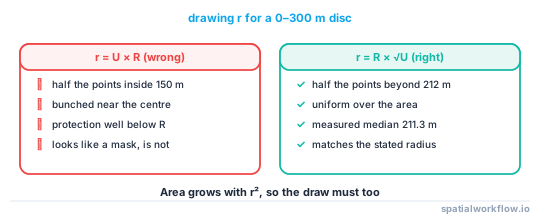
A uniform draw on r concentrates points near the centre, because area grows with r². For a disc use r = R·√U; for an annulus use r = √(U·(r_max² − r_min²) + r_min²). Getting this wrong is the commonest bug in masking code and it silently halves the protection.
2. Work in a projected CRS
Displacement is a distance in metres. Adding degrees to degrees stretches the mask east–west by 1/cos(latitude) — at 50.8°N that is a 37% error, and at 60°N a factor of two. Reproject, mask, reproject back.
3. Choose r_max from a candidate count, not from a feeling
The radius that matters is the one that reaches your target k. On the Brighton addresses the distance to the fifth nearest other address had a median of 21.9 m and a maximum of 533.6 m, so a single 300 m radius over-protects the centre and under-protects the edge. Spatial k-anonymity explained has the calculation.
4. Choose r_min from what a near-miss would reveal
r_min stops a point landing on its own rooftop. Set it above the typical parcel size — 25 m in a dense terrace, 50–100 m in suburbs. Note the cost: publishing r_min tells an attacker where the point is not, which shrinks the candidate set slightly.
5. Constrain the result to plausible ground
A masked point in the sea, in a lake, on an airfield or across an administrative boundary is worse than no mask: it is visibly wrong, and it tells an attacker that the true point is on the land side. Rejection sampling fixes it cheaply — on the Brighton coastal strip, a 50–300 m donut put 63 of 3,109 points in the English Channel, and redrawing them took 3 rounds with a maximum of 4 attempts for a single point.
6. Store the mask, do not regenerate it
If the dataset is published again, publish the same masked coordinates. Sixteen independent redraws of a 50–300 m donut left 59.0% of points within 50 m of the truth once averaged. Keep the masked file, or keep the seed and the code.
7. Report what the mask cost
Publish the method, the radii, the CRS and the measured effect on the statistics people will compute. On these points a 50–300 m donut raised the mean nearest-neighbour distance from 11.8 m to 28.0 m and kept only 43.1% of the top-5% kernel density cells.
Code examples
Example 1 — the three methods side by side
import numpy as np
from scipy.spatial import cKDTree

rng = np.random.default_rng(20260915)

def disc(xy, R):
    th = rng.uniform(0, 2*np.pi, len(xy)); r = R * np.sqrt(rng.uniform(0, 1, len(xy)))
    return xy + np.c_[r*np.cos(th), r*np.sin(th)]

def donut(xy, r0, r1):
    th = rng.uniform(0, 2*np.pi, len(xy))
    r = np.sqrt(rng.uniform(0, 1, len(xy))*(r1**2 - r0**2) + r0**2)
    return xy + np.c_[r*np.cos(th), r*np.sin(th)]

def adaptive(xy, candidates, k=5):
    d, _ = cKDTree(candidates).query(xy, k=k + 1)
    R = d[:, k]
    th = rng.uniform(0, 2*np.pi, len(xy)); r = R * np.sqrt(rng.uniform(0, 1, len(xy)))
    return xy + np.c_[r*np.cos(th), r*np.sin(th)]

for name, out in [("disc 300", disc(xy, 300)),
                  ("donut 50-300", donut(xy, 50, 300)),
                  ("adaptive k=10", adaptive(xy, xy, 10))]:
    d = np.hypot(*(out - xy).T)
    print(f"{name:14} median {np.median(d):6.1f} m  min {d.min():6.1f} m  max {d.max():7.1f} m")
disc 300 median 200.2 m min 8.4 m max 299.9 m
donut 50-300 median 215.0 m min 50.2 m max 300.0 m
adaptive k=10 median 23.6 m min 0.1 m max 580.1 m
The adaptive mask moves the median point an order of magnitude less and still protects the isolated ones, because it spends the displacement where it is needed.
Example 2 — donut sweep with the displacement percentiles that matter
for r0, r1 in [(0, 100), (0, 300), (50, 300), (100, 500)]:
    m = donut(xy, r0, r1)
    d = np.hypot(*(m - xy).T)
    print(f"{r0:4d}-{r1:4d} m: mean {d.mean():6.1f}  median {np.median(d):6.1f}  "
          f"min {d.min():5.1f}  p5 {np.percentile(d, 5):6.1f}")
0- 100 m: mean 65.9 median 70.0 min 1.6 p5 20.7
0- 300 m: mean 200.2 median 211.3 min 8.4 p5 64.3
50- 300 m: mean 204.9 median 215.0 min 50.2 p5 82.5
100- 500 m: mean 345.0 median 358.6 min 100.2 p5 155.4
Read the 5th percentile, not the mean: it is the protection the weakest 5% of points receive.
Example 3 — keeping the mask reproducible
import json, hashlib

PARAMS = {"method": "donut", "r_min": 50, "r_max": 300, "crs": "EPSG:27700", "seed": 20260915}

rng = np.random.default_rng(PARAMS["seed"])
masked = donut_mask(xy, PARAMS["r_min"], PARAMS["r_max"], rng)

PARAMS["output_sha256"] = hashlib.sha256(masked.tobytes()).hexdigest()[:16]
print(json.dumps(PARAMS, indent=2))
Store this next to the release. The seed is not a secret — it is what lets you produce the identical file next year instead of a fresh draw that averages away the protection.
Explanation
Why donut masking exists
Plain perturbation leaves a tail of points that barely move. With a 300 m disc, 5% of points moved less than 64.3 m and the minimum was 8.4 m — a point that has moved 8 m is still on its own property. The inner radius removes that tail at the cost of a small, publishable piece of information about where the point is not.
Why adaptive masking is usually the right default
Fixed-radius masking makes displacement uniform and protection uneven; adaptive masking makes protection uniform and displacement uneven. Since the thing you are promising is protection, uniform protection is what the promise should be about. The cost is that the radius becomes a function of the candidate layer, which must therefore be fixed, documented, and published with the data.
Why masking is weaker than aggregation
A masked release still contains one row per subject. That row can be attacked from another direction — the attributes, the timestamp, a second release, the row order — and every one of those attacks has been used. Aggregation destroys the row. Reach for masking only when the analysis genuinely needs point geometry.
Why the projection matters more than it looks
Masking in EPSG:4326 by adding degrees produces an ellipse, not a circle, and the ellipse is wrong in the direction the data is densest. It also breaks near the poles and across the antimeridian. All masking should happen in a local projected CRS; How to choose a projected CRS for an area covers picking one.
Edge cases or notes
- Mask once per subject, not once per record. Two events at the same house must move together, or the pair of masked points brackets the truth.
- Preserve topology where it is published. If the release also gives a ward, mask within the ward or the counts stop matching.
- Elevation and coastlines constrain the draw. Rejection sampling against a land mask is cheap; a point in the sea is not.
- Do not round after masking. Rounding a masked coordinate to 3 dp adds a grid artefact that is visible on a map.
- Do not mask the derived surfaces separately. Derive them from the masked points, or the two disagree.
- Very small datasets cannot be masked usefully. Twenty points in a village stay identifiable at any radius.
- Publish the parameters. Concealing them adds nothing and prevents users correcting for the induced bias.
- Masked data is still personal data in most jurisdictions. It reduces risk; it does not create anonymity.
Internal links
- Spatial k-anonymity explained — choosing the radius from a candidate count
- How to apply donut geomasking to sensitive points in Python — the full implementation with a land mask
- Geomasked points land in the sea or outside the study area — constraining the draw
- Geomasking changed the result of the analysis — measuring and reporting the cost
- Geoprivacy explained: why coordinates are personal data — when masking is the wrong tool
- Aggregation and suppression rules explained — the alternative that removes the row
- How to choose a projected CRS for an area — masking in metres, not degrees
- How to reduce coordinate precision safely in Python — the cheaper cousin of masking
FAQ
What is geomasking?
Displacing each point by a random amount so that the released location is plausible but not the true one, while the dataset stays usable for analysis at a coarser scale.
What is the difference between random and donut masking?
Donut masking adds a minimum displacement, so no point can stay within r_min of where it started. Plain random perturbation leaves a tail of points that barely moved.
How do I choose the radius?
From the number of candidate subjects it must cover. Compute the distance to the kth nearest dwelling and use that, which in the Brighton test ranged from 21.9 m in the median case to 533.6 m at the extreme for k=5.
Why does my masked point land in the sea?
Because the draw is unconstrained. Reject and redraw against a land mask; on a coastal dataset this affected 63 of 3,109 points and took three rounds to resolve.
Can I re-run the mask each time I publish?
No. Independent redraws average out — after sixteen releases, 59% of points were within 50 m of their true location. Publish the same masked file, or store the seed.
Does masking make the data anonymous?
No. It reduces re-identification risk by a measurable amount, which is a different and weaker claim, and most regulators still treat the result as personal data.