Re-identification risk in spatial data explained

Problem statement

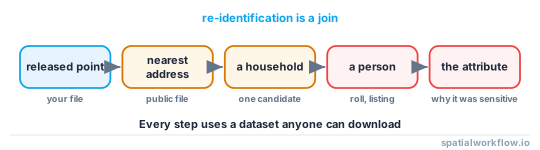
Nobody re-identifies a dot by looking at it. They join it to something. That is the only mechanism, and it is the reason "we removed the names" and "the dots are too small to read" are both irrelevant: the attack happens in a database, not on a map.

The joins are cheap and public. Address files, property listings, electoral rolls, company registers, obituaries, planning applications and OpenStreetMap all contain coordinates or addresses for identifiable people and places. A released point becomes a name as soon as it falls within a few metres of exactly one record in any of them.

What makes this hard to reason about is that risk is not a property of the dataset. It is a property of the dataset plus the auxiliary data plus the number of times you publish. This guide sets out the three in the order they bite, and shows how to put a number on each.

Quick answer

Measure risk as "how many candidates does each released point leave?", using a public address file as the attacker's table:

import numpy as np
from scipy.spatial import cKDTree

tree = cKDTree(np.c_[addresses.geometry.x, addresses.geometry.y])   # attacker's auxiliary data
released_xy = np.c_[released.geometry.x, released.geometry.y]

k = np.array([len(c) for c in tree.query_ball_point(released_xy, 50)])   # candidates within 50 m
print(f"{(k < 5).sum():,} of {len(released):,} points ({(k < 5).mean():.1%}) "
      f"leave fewer than 5 candidates; {(k == 1).sum():,} leave exactly one")

382 of 4,064 points (9.4%) leave fewer than 5 candidates; 69 leave exactly one

Released unmasked, every one of the 4,064 Brighton & Hove OpenStreetMap address points sits exactly on its own address — the worst case by construction, and the case an unmasked release of home locations actually is. Masked once by 50–300 m and checked against all 200,809 UPRNs in the city, most points leave dozens of candidates within 50 m — but 382 (9.4%) leave fewer than five and 69 leave exactly one, and those are the release.

Name the attacker's table, then count candidates

1. Write the attacker's table down explicitly

Risk cannot be computed without naming what the point is joined to. In order of how easily each is obtained:

Coverage changes the answer more than precision does. On the same masked Brighton release, 73.7% of points had fewer than five OpenStreetMap address nodes within 50 m and 9.4% had fewer than five UPRNs (Example 4). An attacker uses the complete file, so the audit has to as well.

2. Count the candidates each point leaves

The quantity to report is the size of the candidate set: how many plausible subjects a released point is consistent with. One is a re-identification. Five is the usual regulatory floor. The number is computed the same way whatever the release method — count the auxiliary records within the release's uncertainty radius.

3. Distinguish population density from address density

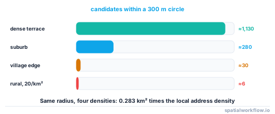
Two released points 200 m apart in a city centre and in a village have wildly different risk, and the variable that explains it is how many possible subjects share the uncertainty area. A fixed masking radius therefore produces uneven protection: the same 300 m circle covers about 3,000 addresses in central Brighton and about twenty on the downland at the city's northern edge (Example 2). Spatial k-anonymity explained is the fix.

4. Check the attributes, not just the geometry

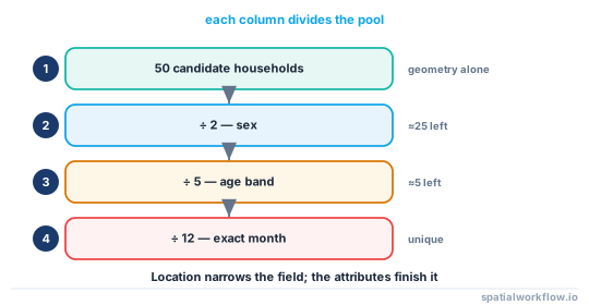
Location narrows the field; attributes finish the job. A released point with age_band, sex and date attached can be unique among the households its geometry is consistent with even when the geometry alone leaves fifty candidates. Treat every published column as part of the key.

5. Check the repeat-release channel

The single most common failure in practice is not a bad first release. It is a second one. Masked points redrawn independently average towards the truth, an updated boundary file lets two aggregations be subtracted, and a monthly series of counts turns one suppressed cell into an arithmetic problem. Decide the release cadence before the method.

6. Check the derived products

A kernel density surface, a hotspot map, an interpolated raster and an SVG export all carry the input points forward in a form that can be inverted. A KDE at a 25 m bandwidth has a local maximum near every input point; an SVG scatter has one <use> element per point with exact coordinates in its attributes.

Candidate sets for points in Brighton & Hove

The data used on this page

Two real files for Brighton & Hove. The released points are every OpenStreetMap node in the city carrying an addr:housenumber (true_xy), donut-masked once by 50–300 m (released). The attacker's table (addresses) is every UPRN inside the city boundary from Ordnance Survey's OS Open UPRN (September 2026 release, 619 MB zipped, Open Government Licence) — the complete, free list of addressable locations in Great Britain. Overpass via the maps.mail.ru mirror, read from its answer of 9 October 2026, which the geoprivacy guides share.

import io
import os
import zipfile

import geopandas as gpd
import numpy as np
import osmnx as ox
import pandas as pd
import requests

# OpenStreetMap as Overpass returned it on 9 October 2026, saved as osmnx's own cache so the counts
# below do not drift as OSM is edited; delete the cache folder to query live instead
if not os.path.exists("cache"):
    reply = requests.get("https://www.spatialworkflow.io/data/osm-cache-brighton-addresses-2026-10-09.zip", timeout=300)
    reply.raise_for_status()
    with zipfile.ZipFile(io.BytesIO(reply.content)) as archive:
        archive.extractall("cache")

ox.settings.overpass_url = "https://maps.mail.ru/osm/tools/overpass/api"
ox.settings.overpass_rate_limit = False
ox.settings.http_user_agent = "spatialworkflow.io guide examples (https://www.spatialworkflow.io/)"
boundary = ox.geocode_to_gdf("Brighton and Hove, England")
features = ox.features_from_polygon(boundary.geometry.iloc[0], tags={"addr:housenumber": True})
nodes = features[features.index.get_level_values(0) == "node"].to_crs(27700)
true_xy = np.c_[nodes.geometry.x, nodes.geometry.y]

rng = np.random.default_rng(20260915)
theta = rng.uniform(0, 2 * np.pi, len(true_xy))
r = np.sqrt(rng.uniform(0, 1, len(true_xy)) * (300**2 - 50**2) + 50**2)
released = gpd.GeoDataFrame(geometry=gpd.points_from_xy(true_xy[:, 0] + r * np.cos(theta),
                                                        true_xy[:, 1] + r * np.sin(theta)), crs=27700)

if not os.path.exists("brighton_uprn.gpkg"):
    if not os.path.exists("osopenuprn_csv.zip"):
        with requests.get("https://api.os.uk/downloads/v1/products/OpenUPRN/downloads"
                          "?area=GB&format=CSV&redirect", stream=True, timeout=600) as reply:
            reply.raise_for_status()
            with open("osopenuprn_csv.zip", "wb") as out:
                for chunk in reply.iter_content(1 << 20):
                    out.write(chunk)
    x0, y0, x1, y1 = boundary.to_crs(27700).total_bounds
    with zipfile.ZipFile("osopenuprn_csv.zip") as z:
        name = next(n for n in z.namelist() if n.endswith(".csv"))
        with z.open(name) as f:
            keep = [c[c.X_COORDINATE.between(x0, x1) & c.Y_COORDINATE.between(y0, y1)]
                    for c in pd.read_csv(f, chunksize=2_000_000)]
    uprn = pd.concat(keep)
    uprn = gpd.GeoDataFrame(uprn[["UPRN"]], crs=27700,
                            geometry=gpd.points_from_xy(uprn.X_COORDINATE, uprn.Y_COORDINATE))
    uprn[uprn.within(boundary.to_crs(27700).geometry.iloc[0])].to_file("brighton_uprn.gpkg")
addresses = gpd.read_file("brighton_uprn.gpkg")
print(f"{len(true_xy):,} OSM address points released; {len(addresses):,} UPRNs in the attacker's table")

4,064 OSM address points released; 200,809 UPRNs in the attacker's table

Example 1 — candidate set size at a given uncertainty radius

import numpy as np
from scipy.spatial import cKDTree

tree = cKDTree(np.c_[addresses.geometry.x, addresses.geometry.y])
released_xy = np.c_[released.geometry.x, released.geometry.y]

for radius in (25, 50, 100, 250, 500):
    k = np.array([len(tree.query_ball_point(p, radius)) for p in released_xy])
    print(f"{radius:4d} m: median candidates {np.median(k):5.0f}, "
          f"points with fewer than 5 candidates {(k < 5).mean():6.1%}")

  25 m: median candidates    13, points with fewer than 5 candidates  28.5%
  50 m: median candidates    68, points with fewer than 5 candidates   9.4%
 100 m: median candidates   317, points with fewer than 5 candidates   2.8%
 250 m: median candidates  2099, points with fewer than 5 candidates   0.1%
 500 m: median candidates  7292, points with fewer than 5 candidates   0.0%

Run it on the release, not on the source. The radius is whatever the masking or rounding guarantees; for an unmasked release it is the coordinate precision.

Example 2 — the same released point in two places

# Two 2 km x 2 km squares (British National Grid), both inside Brighton & Hove
boxes = {"city centre": (530000, 103500, 532000, 105500),     # Brighton station to the seafront
         "downland":    (528000, 108500, 530000, 110500)}     # Patcham fringe and the Downs above it

for name, (x0, y0, x1, y1) in boxes.items():
    inside = addresses.cx[x0:x1, y0:y1]
    density = len(inside) / ((x1 - x0) * (y1 - y0) / 1e6)
    print(f"{name}: {density:,.0f} addresses per km²; "
          f"a 300 m mask covers about {density * np.pi * 0.3**2:,.0f} of them")

city centre: 10,922 addresses per km²; a 300 m mask covers about 3,088 of them
downland: 74 addresses per km²; a 300 m mask covers about 21 of them

A 300 m radius is 0.283 km². At the city centre's 10,922 addresses per km² it hides a point among about 3,088 candidates; at the downland square's 74 per km² it hides it among about 21 — a factor of 150 from one radius, four kilometres apart.

Example 3 — the repeat-release attack, measured

import numpy as np
from scipy.spatial import cKDTree

rng = np.random.default_rng(3)

def donut(xy, rmin, rmax):
    theta = rng.uniform(0, 2 * np.pi, len(xy))
    r = np.sqrt(rng.uniform(0, 1, len(xy)) * (rmax**2 - rmin**2) + rmin**2)
    return xy + np.c_[r * np.cos(theta), r * np.sin(theta)]

tree = cKDTree(true_xy)
acc = np.zeros_like(true_xy)
for i in range(1, 17):
    acc += donut(true_xy, 50, 300)          # a fresh mask each month
    est = acc / i
    err = np.hypot(*(est - true_xy).T)
    if i in (1, 2, 4, 8, 16):
        print(f"{i:2d} releases: median error {np.median(err):6.1f} m, "
              f"within 50 m {(err < 50).mean():5.1%}")

 1 releases: median error  214.0 m, within 50 m  0.0%
 2 releases: median error  138.0 m, within 50 m  9.3%
 4 releases: median error   92.8 m, within 50 m 17.4%
 8 releases: median error   63.6 m, within 50 m 34.4%
16 releases: median error   45.0 m, within 50 m 57.7%

Example 4 — the numbers behind the density figure

uprn_tree = cKDTree(np.c_[addresses.geometry.x, addresses.geometry.y])
k300 = np.array([len(c) for c in uprn_tree.query_ball_point(released_xy, 300)])
print(f"candidates within 300 m of the {len(released_xy):,} masked points: "
      f"max {k300.max():,}, 90th pct {np.percentile(k300, 90):,.0f}, median {np.median(k300):,.0f}, "
      f"10th pct {np.percentile(k300, 10):,.0f}, min {k300.min():,}")
osm_tree = cKDTree(true_xy)
k_osm = np.array([len(c) for c in osm_tree.query_ball_point(released_xy, 50)])
k_uprn = np.array([len(c) for c in uprn_tree.query_ball_point(released_xy, 50)])
print(f"fewer than 5 within 50 m: {(k_osm < 5).mean():.1%} against OSM, {(k_uprn < 5).mean():.1%} against UPRN")

candidates within 300 m of the 4,064 masked points: max 6,996, 90th pct 4,665, median 2,975, 10th pct 717, min 9
fewer than 5 within 50 m: 73.7% against OSM, 9.4% against UPRN

Sixteen monthly releases of the same 4,064 Brighton points, each masked to 50–300 m, put 57.7% of them within 50 m of the truth. Mask once and store the mask, or the protection decays as 1/√n.

Why candidate-set size is the right number

Why candidate-set size is the right number

Probability of re-identification is hard to defend, because it depends on assumptions about the attacker. Candidate-set size is a count you can compute from public data and state without modelling anyone's intentions: "each released point is consistent with at least k addresses". It is also what regulators ask for, under the name k-anonymity.

Why partial auxiliary data gives the wrong answer

OpenStreetMap holds 4,064 address nodes in Brighton & Hove; OS Open UPRN holds 200,809 addressable locations inside the same boundary. Measured against the partial file, a candidate count is too small and the release looks riskier than it is — 73.7% of masked points failing at 50 m instead of 9.4%. That is not a safe error to make either: it points the effort at the wrong records, and it gives no reason to trust the ones that pass. Use the most complete file you can get, which is the one an attacker will use, and say which one you used.

Why attributes multiply rather than add

Location leaves k candidates; an attribute that splits the population into m roughly equal groups leaves about k/m. Two or three such attributes will finish off a candidate set of fifty. This is why a "low-risk" geometry combined with date of birth and sex is not low risk, and it is the same arithmetic that made a US voter roll re-identify medical records in the 1990s.

Why derived surfaces are not safer than points

Smoothing is not destruction. A kernel density estimate is a sum of kernels centred on the inputs; with a known bandwidth, the inputs can be recovered approximately by deconvolution, and with a small bandwidth they can be read off the local maxima. Publish the surface at a bandwidth that is at least as large as the protection you claim, and clamp the cell size to match.

Outliers, subgroups, time and colleagues

• Uniqueness is not symmetric. A point that matches one address is a re-identification; an address that matches one point is not necessarily.
• Outliers leak first. The most isolated 1% of points carry most of the risk and are usually the ones a fixed radius fails to protect.
• Small subgroups fail everywhere. A rare category can be unique within a whole city.
• Time is a quasi-identifier. An exact timestamp plus a neighbourhood is often unique.
• The "attacker" is often a colleague. Most real re-identifications are casual recognition by someone who knows the area.
• Re-identification does not require certainty. A 1-in-3 guess is harmful if the attribute is sensitive enough.
• Geocoded addresses inherit the geocoder's bias. Interpolated street-segment matches leave larger candidate sets than rooftop matches, so risk varies by how the data was geocoded.
• Publishing the method is still correct. Security by obscurity fails here as everywhere; publish the parameters and rely on them being sufficient.

Internal links

• Geoprivacy explained: why coordinates are personal data — why the geometry column is the identifier
• Spatial k-anonymity explained — turning candidate-set size into a rule
• How to measure re-identification risk in a point dataset — the full audit script
• Geomasking methods explained: donut, random and adaptive — what a masking radius does and does not buy
• Anonymised points still identify individuals — the failures this measurement predicts
• Differential privacy for spatial counts explained — the defence designed for repeat queries
• How to geocode addresses in Python — where the auxiliary data comes from
• Kernel density estimation explained — why a density surface still contains the points

FAQ

What is re-identification, exactly?

Linking a record in a de-identified release back to the individual it describes, usually by joining it to another dataset that contains both the same quasi-identifiers and a name.

How do I measure risk without the attacker's data?

Use the most complete public address file you can get — in Great Britain, OS Open UPRN is free — and report which one you used. OpenStreetMap is a poor substitute where its address coverage is thin: in Brighton & Hove it has about one node for every 50 UPRNs.

Does masking to 300 m make a point safe?

It depends entirely on how many possible subjects live within 300 m. Across the masked Brighton points the count ran from 9 to 6,996 addresses, with a median of 2,975.

Why is publishing monthly worse than publishing once?

Independent masks average out. After sixteen monthly releases of the same points, 57% were within 50 m of their true location in the test above.

Do attributes matter if the geometry is protected?

Yes. Each additional published attribute divides the candidate set, and two or three ordinary demographic fields will reduce fifty candidates to one.

Is a heat map safe to publish?

Only if the bandwidth is at least as large as the spatial protection you are claiming. At a small bandwidth the surface has a maximum at every input point.