
Geomasking changed the result of the analysis
Problem statement
The masked dataset went out, somebody ran the analysis they had run on the unmasked version, and the answer was different. The hotspots moved. The nearest-neighbour statistic said the points were no longer clustered. The counts per ward did not match the counts you published.
This is not a bug. Masking adds a known amount of random error to every coordinate, and every spatial statistic is a function of those coordinates. What is a bug is shipping the masked data without saying how much it moved, so that users treat masked results as unmasked ones.
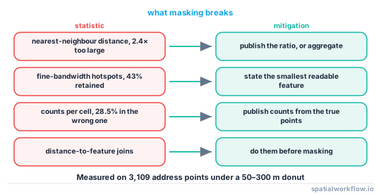
On 3,109 real address points, a 50–300 m donut mask raised the mean nearest-neighbour distance from 11.8 m to 28.0 m, left only 43.1% of the top-5% kernel density cells in the top 5%, and moved 28.5% of points into a different 500 m cell.
Quick answer
Measure the distortion for the statistics your users will compute, and publish the table:
import numpy as np
from scipy.spatial import cKDTree
from scipy.stats import spearmanr

def distortion(true_xy, masked_xy, grid, bw=0.05):
    nn_t = cKDTree(true_xy).query(true_xy, k=2)[0][:, 1]
    nn_m = cKDTree(masked_xy).query(masked_xy, k=2)[0][:, 1]
    kde_t, kde_m = kde(true_xy, grid, bw), kde(masked_xy, grid, bw)
    top = kde_t >= np.percentile(kde_t, 95)
    return {
        "mean_nn_ratio": nn_m.mean() / nn_t.mean(),
        "kde_spearman": spearmanr(kde_t, kde_m).statistic,
        "top5_retained": float(((kde_m >= np.percentile(kde_m, 95)) & top).sum() / top.sum()),
    }
Publish it next to the data. A user who knows the nearest-neighbour statistic is inflated 2.4× can correct for it; a user who does not will report the inflation as a finding.
Step-by-step solution
1. Measure the damage across the radius range
The full curve on the Brighton address points:
| mask | mean NN distance | ratio to truth | KDE ρ (fine) | KDE ρ (coarse) | top-5% cells kept |
|---|---|---|---|---|---|
| none | 11.8 m | 1.000 | 1.0000 | 1.0000 | 100.0% |
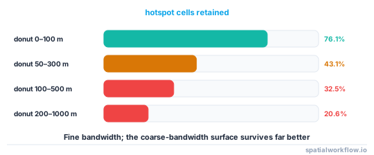
| donut 0–100 m | 20.7 m | 1.758 | 0.9604 | 0.9974 | 76.1% |
| donut 50–300 m | 28.0 m | 2.379 | 0.7946 | 0.9510 | 43.1% |
| donut 100–500 m | 32.0 m | 2.719 | 0.6503 | 0.8564 | 32.5% |
| donut 200–1000 m | 40.5 m | 3.441 | 0.4742 | 0.6477 | 20.6% |
Even the smallest mask nearly doubles the nearest-neighbour statistic. The coarse-bandwidth density survives far better than the fine one, which is the clue to the mitigation.
2. Check the aggregate counts separately
Masking moves points across cell boundaries, so any count computed from the masked points differs from the true one:
| mask | cells | mean absolute error per cell | points in the wrong cell |
|---|---|---|---|
| donut 0–100 m | 66 | 4.3 | 9.1% |
| donut 50–300 m | 69 | 12.8 | 28.5% |
| donut 200–1000 m | 112 | 25.8 | 92.8% |
3. Publish the aggregates yourself
The fix for the count mismatch is not a better mask. It is to compute the aggregates from the true points, publish those, and mask only the point layer — so users take counts from the table and pattern from the points.
4. Constrain the mask to the reporting unit
If the release includes a region column, masking within the region keeps every published total exact. The cost is that the region is disclosed, which it already was.
5. Match the analysis scale to the mask
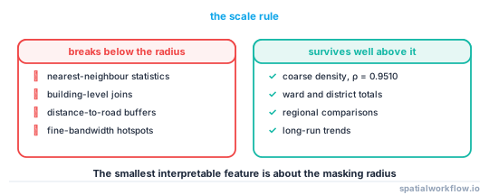
A mask of radius R destroys structure below roughly R and preserves structure well above it. Tell users the resolution the data supports: "do not interpret features smaller than 500 m". The coarse-bandwidth density above kept ρ=0.9510 under the same mask that took the fine one to 0.7946.
6. Use an adaptive radius where accuracy matters most
An adaptive mask spends displacement where candidates are scarce, so dense areas — usually the interesting ones — barely move. Median displacement at k=10 was 23.6 m against 215.0 m for the fixed 50–300 m donut, for the same candidate-count guarantee.
7. Correct the statistics where a correction exists
For some statistics the bias is analytic. Masking adds independent noise of known variance, so second-moment measures can be deconvolved; a K-function or a variogram can have the noise variance subtracted. Publish the noise variance so users can do it.
Code examples
Example 1 — the full distortion sweep
import numpy as np
from scipy.spatial import cKDTree
from scipy.stats import gaussian_kde, spearmanr

gx, gy = np.meshgrid(np.linspace(xy[:, 0].min(), xy[:, 0].max(), 120),
                     np.linspace(xy[:, 1].min(), xy[:, 1].max(), 120))
grid = np.vstack([gx.ravel(), gy.ravel()])

def kde(points, bw):
    return gaussian_kde(points.T, bw_method=bw)(grid)

truth = {bw: kde(xy, bw) for bw in (0.05, 0.15)}
base_nn = cKDTree(xy).query(xy, k=2)[0][:, 1]

for label, (r0, r1) in [("donut 0-100", (0, 100)), ("donut 50-300", (50, 300)),
                        ("donut 100-500", (100, 500)), ("donut 200-1000", (200, 1000))]:
    m = donut(xy, r0, r1)
    nn = cKDTree(m).query(m, k=2)[0][:, 1]
    row = [f"{label:14}", f"{nn.mean():6.1f}", f"{nn.mean() / base_nn.mean():6.3f}"]
    for bw in (0.05, 0.15):
        row.append(f"{spearmanr(truth[bw], kde(m, bw)).statistic:8.4f}")
    print("  ".join(row))
donut 0-100 20.7 1.758 0.9604 0.9974
donut 50-300 28.0 2.379 0.7946 0.9510
donut 100-500 32.0 2.719 0.6503 0.8564
donut 200-1000 40.5 3.441 0.4742 0.6477
Example 2 — counts from the truth, points from the mask
import geopandas as gpd

# Aggregate the true points and publish that table
true_counts = gpd.sjoin(true_points, wards, predicate="within") \
                 .groupby("ward").size().rename("cases")

# Mask within each ward so the masked points also fall in the right one
masked = mask_within_regions(true_points, wards, r_min=50, r_max=300)
masked_counts = gpd.sjoin(masked, wards, predicate="within").groupby("ward").size()

assert (true_counts == masked_counts.reindex(true_counts.index, fill_value=0)).all()
The assertion is the point: if masking is constrained to the reporting units, the published table and the published points agree exactly, and users stop filing bug reports.
Example 3 — the statement to ship with the data
import json

statement = {
    "method": "donut geomask, land-constrained, per-ward",
    "r_min_m": 50, "r_max_m": 300,
    "effect": {
        "mean_nearest_neighbour_ratio": 2.379,
        "kde_spearman_fine_bandwidth": 0.7946,
        "kde_spearman_coarse_bandwidth": 0.9510,
        "top5_density_cells_retained": 0.431,
        "points_in_a_different_500m_cell": 0.285,
    },
    "guidance": "Do not interpret features smaller than about 500 m. "
                "Ward totals are published separately and are exact.",
}
print(json.dumps(statement, indent=2))
Explanation
Why nearest-neighbour statistics break first
Masking adds error of the order of the radius, so any statistic computed at a scale smaller than the radius is dominated by it. The mean nearest-neighbour distance on these addresses was 11.8 m — twenty-five times smaller than the mask — so the measured value afterwards is essentially the mask, not the data. Anything based on short distances (clustering indices, duplicate detection, building-level joins) is in the same position.
Why coarse density survives and fine density does not
A kernel density estimate at bandwidth h is a smoothed version of the point pattern. Masking with radius R convolves the pattern with a second kernel of roughly that width. When h ≫ R, the extra convolution barely changes the result: ρ = 0.9510 at the coarse bandwidth. When h ≈ R, the two are comparable and the surface changes: ρ = 0.7946. The rule of thumb is that the smallest interpretable feature is about the mask radius.
Why the counts must come from the unmasked data
There is no masking radius small enough to keep points in their original cells and large enough to protect them — 9.1% of points crossed a 500 m boundary under a 100 m mask. Either constrain the mask to the units, or publish the counts separately. Doing neither guarantees that the two published products contradict each other.
Why the statement matters as much as the method
A masked dataset with no accuracy statement will be used as if it were exact, and the first result anyone publishes from it will be wrong in a way that is attributable to you. The table above takes an afternoon to compute and removes that entire class of problem.
Edge cases or notes
- Hotspot tests inflate their false-positive rate. Masking flattens peaks; significance thresholds calibrated on unmasked data no longer hold.
- Distance-to-feature analyses are badly hit. "Within 100 m of a road" is meaningless under a 300 m mask.
- Point-in-polygon joins move. Any attribute enriched after masking is enriched from the wrong polygon.
- Interpolation smooths twice. A surface built from masked points is smoother than its stated bandwidth.
- Pair counts are inflated at short range. Ripley's K is biased downward near zero.
- Small samples are affected more. With few points, one displacement changes the statistic.
- The mask variance is publishable. For a donut it is a closed form, and users can deconvolve with it.
- Aggregations coarser than the radius are safe. That is the one thing you can promise without caveat.
Internal links
- Geomasking methods explained: donut, random and adaptive — choosing the radius with this cost in mind
- How to apply donut geomasking to sensitive points in Python — the implementation, including per-region masking
- Spatial k-anonymity explained — the adaptive radius that costs far less accuracy
- Kernel density explained — bandwidth and what it can resolve
- KDE bandwidth is wrong — choosing h for masked data
- The modifiable areal unit problem explained — the other reason counts move
- How to find hotspots with Getis-Ord in Python — the test whose false-positive rate changes
- Geoprivacy explained: why coordinates are personal data — when to aggregate instead of masking
FAQ
How much does geomasking change my results?
It depends on the radius and the statistic. A 50–300 m mask on real address points raised the mean nearest-neighbour distance 2.4×, kept 43.1% of the top-5% density cells and moved 28.5% of points into a different 500 m cell.
Why do my masked counts not match the published totals?
Because masking moves points across boundaries. Publish counts computed from the true points, and constrain the mask to the reporting units if the points must also aggregate correctly.
Which analyses survive masking?
Anything computed at a scale well above the radius. Coarse density kept a rank correlation of 0.9510 under a mask that took the fine-bandwidth version to 0.7946.
Can I correct for the bias?
Partly. The mask adds independent noise of known variance, so second-moment statistics such as variograms and K-functions can be corrected if you publish the variance.
Is there a mask that does not distort anything?
No. Every displacement changes every statistic. What you can choose is where the error goes — an adaptive radius puts it in sparse areas and leaves dense ones nearly intact.
What should I publish alongside masked points?
The method and parameters, the measured distortion for the common statistics, the exact aggregate counts, and a plain statement of the smallest feature users should interpret.