
How to Interpolate Air Quality Station Data in Python
On this page
Problem statement
A city has seventeen NO2 monitors and a question about every street: what is the annual mean here? Interpolation is the obvious answer and a risky one. Seventeen points is very few for a surface that varies by a factor of five within a few hundred metres of a main road; half of the points are kerbside stations that describe their own street and nothing else; and the error of the result is invisible on the map unless it is measured.
The workable recipe has three parts: interpolate only the stations that represent an area, test the interpolation by leaving each station out in turn, and test it against a model field such as CAMS — which, in Berlin, turns out to predict the background better than the stations can.
Quick answer
Annual means for background stations, inverse-distance weighting, and leave-one-out validation:
import io, requests, numpy as np, pandas as pd, geopandas as gpd

API = "https://eeadmz1-downloads-api-appservice.azurewebsites.net/ParquetFile/urls"
META = "https://discomap.eea.europa.eu/map/fme/metadata/PanEuropean_metadata.csv"

r = requests.post(API, json={"countries": ["DE"], "cities": ["Berlin"], "pollutants": ["NO2"],
                             "dataset": 2, "dateTimeStart": "2023-01-01T00:00:00Z",
                             "dateTimeEnd": "2023-12-31T23:00:00Z", "aggregationType": "hour"},
                  timeout=120)
rows = []
for url in [u.strip() for u in r.text.splitlines()[1:] if u.strip()]:
    d = pd.read_parquet(io.BytesIO(requests.get(url, timeout=120).content))
    d["Value"] = pd.to_numeric(d.Value, errors="coerce")
    y = d[(d.Start >= "2023-01-01") & (d.Start < "2024-01-01") & (d.Validity > 0)]
    if len(y) >= 0.9 * 8760:
        rows.append((d.Samplingpoint.iloc[0].split("/")[1], y.Value.mean()))
meta = pd.read_csv(META, sep="\t", low_memory=False,
                   storage_options={"User-Agent": "spatialworkflow-examples/1.0"}).drop_duplicates("SamplingPoint")   # EEA refuses Python's default agent
st = pd.DataFrame(rows, columns=["SamplingPoint", "no2"]).merge(meta, on="SamplingPoint")
st = gpd.GeoDataFrame(st, geometry=gpd.points_from_xy(st.Longitude, st.Latitude),
                      crs=4326).to_crs(25833)
xy = np.c_[st.geometry.x, st.geometry.y]

def idw(xy_known, z_known, xy_query, power=2):
    d = np.hypot(*(xy_query[:, None, :] - xy_known[None, :, :]).transpose(2, 0, 1))
    w = 1 / np.maximum(d, 1.0) ** power
    return (w * z_known).sum(axis=1) / w.sum(axis=1)

def loo(mask_train, mask_test, z):
    errors = []
    for i in np.where(mask_test)[0]:
        train = mask_train.copy()
        train[i] = False
        errors.append(idw(xy[train], z[train], xy[[i]])[0] - z[i])
    return np.array(errors)

z = st.no2.to_numpy()
bg = (st.AirQualityStationType == "background").to_numpy()
for label, train in (("background stations only", bg), ("all stations", np.ones_like(bg))):
    e = loo(train, bg, z)
    print(f"IDW from {label:<25} → error at background sites: "
          f"RMSE {np.sqrt((e ** 2).mean()):.1f}, bias {e.mean():+.1f} µg/m³")
IDW from background stations only → error at background sites: RMSE 4.0, bias +2.0 µg/m³
IDW from all stations → error at background sites: RMSE 9.1, bias +8.6 µg/m³
Evaluated where a background surface should be right — at the background stations — adding the kerbside stations makes it worse, and biased upwards. They pull the surface towards concentrations that exist only next to their roads.
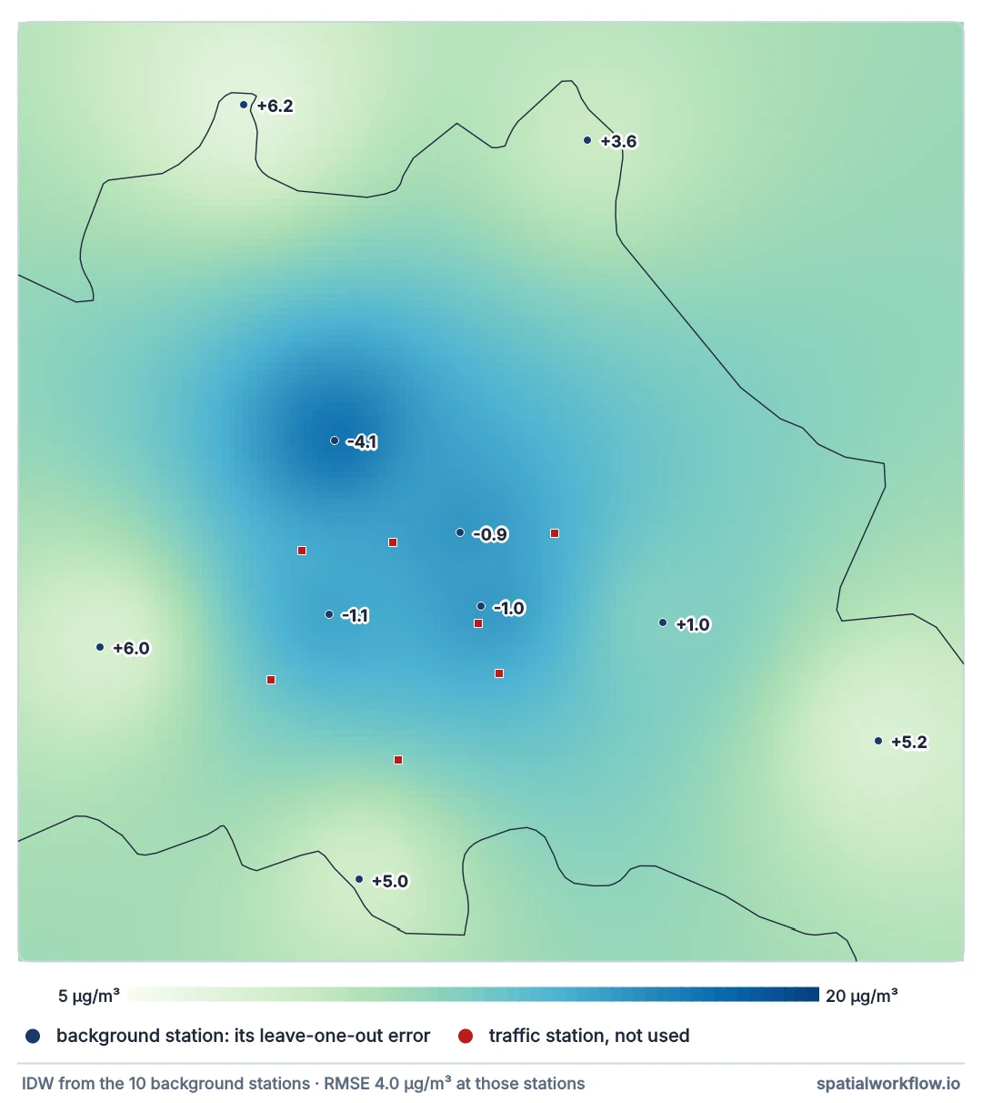
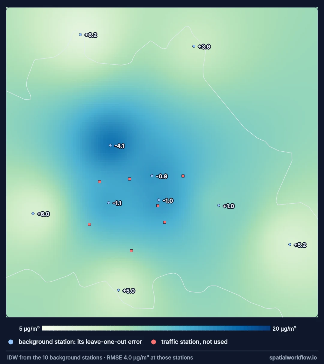
Decide the surface, annual means, metric CRS, leave-one-out
1. Decide what surface you are mapping
Urban background NO2 is a smooth field that interpolation can represent. Roadside NO2 is a network of sharp peaks along streets that it cannot. Choose one; for the other, use a land-use regression or a dispersion model.
2. Compute annual means with a capture threshold
Stations below about 90% capture have biased means. Drop them or flag them before interpolating.
3. Work in a metric CRS
Distances for weights, variograms or kernels must be in metres. For Berlin, ETRS89 / UTM 33N (EPSG:25833).
4. Validate by leaving each station out
With few stations there is no spare data for a test set. Leave one out, predict it from the others, repeat, and report the root-mean-square error and the bias. Without this number the map has no stated accuracy.
5. Give the interpolation a trend
A chemistry-transport model like CAMS knows where the emissions and the wind are, at 10 km or so. Compare it with the interpolation under the same leave-one-out test, and try interpolating the station-minus-model residuals. Whichever wins the test is the surface to publish.
6. Map the uncertainty, not just the value
Show where the surface is supported by a nearby station and where it is extrapolation. IDW has no variance; kriging does, and a simple distance-to-nearest-station layer is better than nothing.
A CAMS trend surface and a gridded map
Example 1 — CAMS as a trend surface
lat, lon = st.Latitude.round(4).tolist(), st.Longitude.round(4).tolist()
j = requests.get("https://air-quality-api.open-meteo.com/v1/air-quality", params={
    "latitude": ",".join(map(str, lat)), "longitude": ",".join(map(str, lon)),
    "hourly": "nitrogen_dioxide", "start_date": "2023-01-01", "end_date": "2023-12-31",
    "domains": "cams_europe"}, timeout=300).json()
st["cams"] = [np.nanmean(np.array(p["hourly"]["nitrogen_dioxide"], dtype=float)) for p in j]

print(st.groupby("AirQualityStationType")[["no2", "cams"]].mean().round(1).to_string())
resid = (st.no2 - st.cams).to_numpy()
e = loo(bg, bg, resid)
print(f"\nCAMS alone at background sites: RMSE "
      f"{np.sqrt(((st.cams - st.no2)[bg] ** 2).mean()):.1f} µg/m³")
print(f"CAMS + IDW of residuals:        RMSE {np.sqrt((e ** 2).mean()):.1f}, "
      f"bias {e.mean():+.1f} µg/m³")
no2 cams
AirQualityStationType
background 11.5 11.1
traffic 24.6 13.1
CAMS alone at background sites: RMSE 2.4 µg/m³
CAMS + IDW of residuals: RMSE 2.5, bias +1.1 µg/m³
The model field alone predicts the background stations with an RMSE of 2.4 µg/m³ — better than IDW from the stations themselves (4.0), with no station information at all. Interpolating its residuals does not help (2.5): with ten stations the residuals are noise rather than a field. And the table shows the model's limit: at the kerbside stations CAMS gives 13.1 against a measured 24.6. At 10 km it sees the city, not its roads. One caution before crediting the model: the CAMS European system assimilates surface observations into each forecast's starting state, and Berlin's network is among them, so leaving a station out of the interpolation does not leave it out of the model. The comparison is fair to the interpolation and generous to CAMS. Even so, the model's field carries structure that ten stations cannot, and the right role for the stations here is to check it, not to replace it.
Example 2 — a surface on a grid
x0, y0, x1, y1 = st.total_bounds
gx, gy = np.meshgrid(np.arange(x0, x1, 500), np.arange(y0, y1, 500))
grid = np.c_[gx.ravel(), gy.ravel()]
surf_bg = idw(xy[bg], z[bg], grid)
surf_all = idw(xy, z, grid)
print(f"grid: {gx.shape[1]} × {gx.shape[0]} cells of 500 m")
print(f"background-only surface: {surf_bg.min():.1f}–{surf_bg.max():.1f} µg/m³, "
      f"median {np.median(surf_bg):.1f}")
print(f"all-station surface:     {surf_all.min():.1f}–{surf_all.max():.1f} µg/m³, "
      f"median {np.median(surf_all):.1f}")
print(f"cells where including traffic stations adds > 5 µg/m³: "
      f"{(surf_all - surf_bg > 5).mean():.0%}")
grid: 58 × 57 cells of 500 m
background-only surface: 6.7–17.5 µg/m³, median 11.8
all-station surface: 6.8–31.5 µg/m³, median 16.9
cells where including traffic stations adds > 5 µg/m³: 39%
The all-station surface has a median of 16.9 against 11.8, and 39% of cells gain more than 5 µg/m³ — not only near the kerbside stations. IDW spreads each station's value over the space between stations, and seven of them are roads.
Example 3 — how far is each cell from its evidence?
from scipy.spatial import cKDTree

dist, _ = cKDTree(xy[bg]).query(grid)
print(f"distance to the nearest background station: median {np.median(dist) / 1000:.1f} km, "
      f"90th percentile {np.percentile(dist, 90) / 1000:.1f} km")
print(f"share of cells more than 5 km from any background station: {(dist > 5000).mean():.0%}")
distance to the nearest background station: median 4.6 km, 90th percentile 8.1 km
share of cells more than 5 km from any background station: 44%
That layer belongs on the map next to the surface. Where the nearest station is several kilometres away, the value is mostly the weighting scheme's opinion.
IDW over kriging, and background-only validation
Why IDW and not kriging here
Kriging needs a variogram, and a variogram needs pairs of stations at many separations. Ten background stations give 45 pairs — too few to estimate one reliably. IDW has no model to get wrong, and leave-one-out validation says how well it does. With a few dozen stations, ordinary or universal kriging becomes worthwhile, mainly for its variance estimate.
Why residual interpolation did not help
Residual interpolation pays when the model is wrong in a spatially coherent way — too low across the whole east of a city, say — because then neighbouring stations share the error and can correct it. Here the residuals are small and uncorrelated between stations a few kilometres apart, so interpolating them adds noise. With a denser network, or a model with a known regional bias, the result can go the other way; the leave-one-out test is how you find out.
Why validation at background sites only
The surface claims to be the urban background. Testing it at kerbside stations would penalise it for not predicting what it deliberately excludes, and reward a surface contaminated by them for predicting roads badly everywhere else.
Duplicate points, edges and the power parameter
- Duplicate sampling points at one station must be averaged or one chosen before interpolation.
- Edge effects: IDW flattens towards the mean outside the station hull; clip the map to where stations are.
- Power parameter: higher powers make bullseyes sharper; choose it by leave-one-out RMSE, not by eye.
- CAMS domains: the European ensemble is about 10 km; the global model is much coarser.
- Temporal mismatch: build annual means from the same hours for model and stations if either has gaps.
Internal links
- Air quality monitoring networks explained — why background and traffic differ
- Interpolated pollution map shows bullseyes — the fix guide for mixed stations
- How to build a land-use regression model for NO2 — mapping the roadside part
- How to cross-validate an interpolation — validation in general
- How to krige in Python — when there are enough stations for a variogram
- How to calculate population-weighted exposure — using the surface
FAQ
How do I interpolate air quality monitoring data?
Use background stations only, interpolate annual means in a metric CRS, and validate with leave-one-out cross-validation.
Should I include traffic stations?
Not in a background surface. They represent their street, not the space between stations.
Is kriging better than IDW?
With a few dozen well-spread stations, usually, and it gives a variance. With ten, the variogram cannot be estimated reliably.
How do I know how accurate my pollution map is?
Leave each station out, predict it from the rest, and report the RMSE and bias.
Can I use a model to improve interpolation?
Test it: in Berlin the CAMS field alone beat station interpolation. Interpolating station-minus-model residuals helps only when the model's errors are spatially coherent.
What is CAMS?
The Copernicus Atmosphere Monitoring Service, which publishes modelled air quality over Europe at about 10 km, available through Open-Meteo's air quality API.