Air Quality Monitoring Networks Explained

On this page

Problem statement

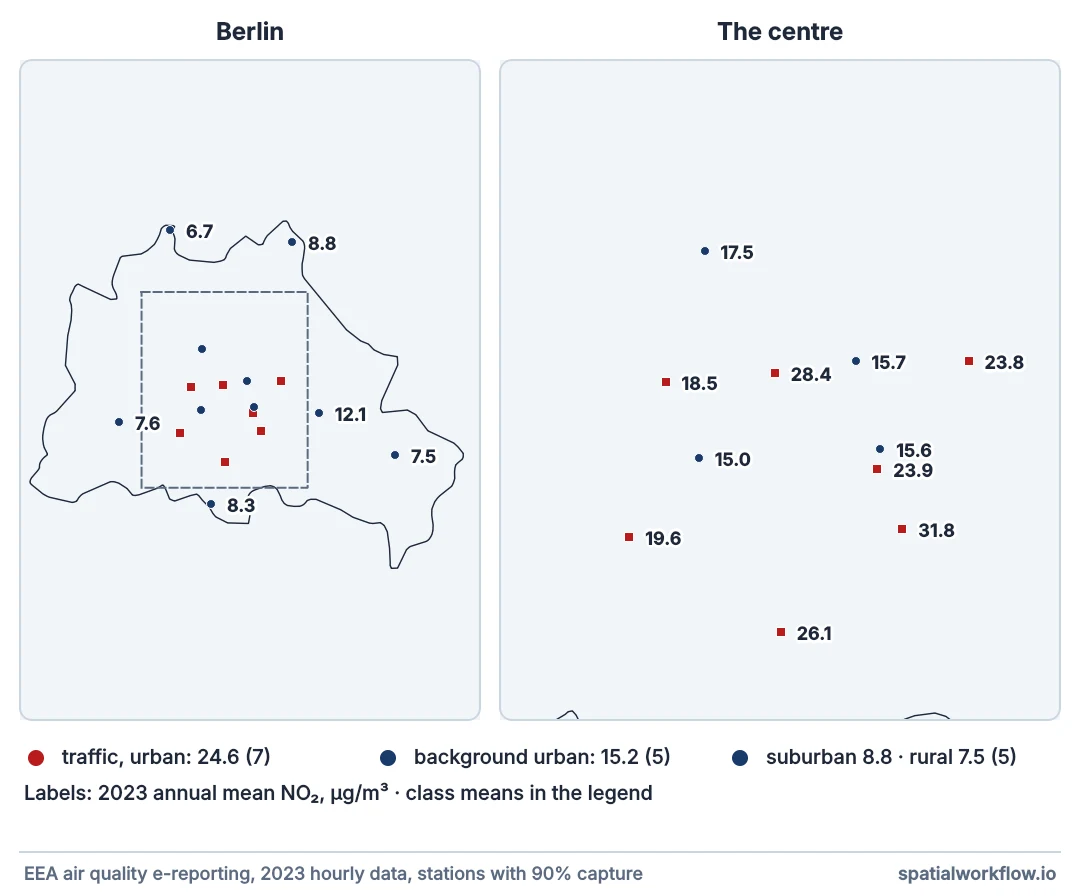
A city's monitoring network looks like a sample of its air: seventeen points, seventeen annual means, average them and you have the city. It is not a sample. Stations are placed by rule to answer specific questions — where are the worst concentrations people are exposed to, what is the general level in residential areas, what arrives from outside the city — and each kind of station is deliberately unrepresentative of the others.

Berlin's NO2 network makes the point in one table. The traffic stations average more than twice the background ones. Which "Berlin average" a report quotes depends on which rows it includes, and a map interpolated across all of them draws the city's side streets with the concentrations of its busiest kerbs.

Quick answer

Every European station is classified along two axes, and both are in the EEA metadata:

Station type — traffic (dominated by a nearby road), industrial, or background (not dominated by any single source).
Station area — urban, suburban, rural, rural-nearcity, and so on.

import io, requests, pandas as pd

API = "https://eeadmz1-downloads-api-appservice.azurewebsites.net/ParquetFile/urls"
META = "https://discomap.eea.europa.eu/map/fme/metadata/PanEuropean_metadata.csv"

def eea_urls(country, city, pollutant):
    r = requests.post(API, json={"countries": [country], "cities": [city],
                                 "pollutants": [pollutant], "dataset": 2,
                                 "dateTimeStart": "2023-01-01T00:00:00Z",
                                 "dateTimeEnd": "2023-12-31T23:00:00Z",
                                 "aggregationType": "hour"}, timeout=120)
    return [u.strip() for u in r.text.splitlines()[1:] if u.strip()]

def annual_mean(url, year=2023):
    d = pd.read_parquet(io.BytesIO(requests.get(url, timeout=120).content))
    d["Value"] = pd.to_numeric(d["Value"], errors="coerce")
    y = d[(d.Start >= f"{year}-01-01") & (d.Start < f"{year + 1}-01-01") & (d.Validity > 0)]
    return d.Samplingpoint.iloc[0].split("/")[1], y.Value.mean(), len(y) / 8760

meta = pd.read_csv(META, sep="\t", low_memory=False,
                   storage_options={"User-Agent": "spatialworkflow-examples/1.0"})   # EEA refuses Python's default agent
rows = [annual_mean(u) for u in eea_urls("DE", "Berlin", "NO2")]
st = (pd.DataFrame(rows, columns=["SamplingPoint", "no2", "capture"])
        .merge(meta[["SamplingPoint", "AirQualityStationType", "AirQualityStationArea",
                     "KerbDistance", "Longitude", "Latitude"]].drop_duplicates("SamplingPoint"),
               on="SamplingPoint"))
st = st[st.capture >= 0.9]
print(st.groupby(["AirQualityStationType", "AirQualityStationArea"])["no2"]
        .agg(["count", "mean", "min", "max"]).round(1).to_string())

                                             count  mean   min   max
AirQualityStationType AirQualityStationArea                         
background            rural-nearcity             4   7.5   6.7   8.3
                      suburban                   1   8.8   8.8   8.8
                      urban                      5  15.2  12.1  17.5
traffic               urban                      7  24.6  18.5  31.8

Each class is a distinct population of sites. The traffic stations are not noisier background stations; they measure a different thing.

Two maps of Berlin’s NO2 monitoring stations: the whole city on the left and the centre enlarged on the right. Traffic stations, drawn as red squares, are all in the centre and read 18.5 to 31.8; background stations, drawn as blue circles, spread out to the edges and read 6.7 to 17.5. — Berlin’s 17 stations with 90% data in 2023, labelled with their annual mean. The seven traffic stations are all in the inner city and read 18.5 to 31.8 µg/m³; the background stations spread out to the edge, where the rural-nearcity ones read 6.7 to 8.3. Where a station stands is part of what it measures.

Station classification first, then match the question

1. Read the station classification before the values

Type and area are part of the observation. A value with no station type is uninterpretable for anything spatial.

2. Know why traffic stations exist

European rules require stations where the highest concentrations to which the population is exposed are expected — usually a kerb on a busy street. They exist to check compliance at the worst places, not to describe the average.

3. Match the station type to the question

Population exposure across a city: urban and suburban background. Compliance at hotspots: traffic. Regional transport and what the city adds: rural background upwind and downwind. Mixing them answers none of these.

4. Check representativeness

A traffic station represents a stretch of street of perhaps 100 m; an urban background station a few square kilometres; a rural station hundreds. Interpolating between stations assumes each represents the space between them, which is only true for background stations.

5. Watch for sentinels in the metadata

KerbDistance of -999 means "not applicable" (background stations) or "unknown", not a distance. Filter or replace sentinels before using them as numbers.

Each station type answers a different question and represents a different area.

Four defensible averages for Berlin

Example 1 — which Berlin average?

print(f"all {len(st)} stations:        {st.no2.mean():.1f} µg/m³")
for label, sel in (("background only", st.AirQualityStationType == "background"),
                   ("urban background", (st.AirQualityStationType == "background")
                                         & (st.AirQualityStationArea == "urban")),
                   ("traffic only", st.AirQualityStationType == "traffic")):
    print(f"{label + ':':<22}{st[sel].no2.mean():>6.1f} µg/m³  ({sel.sum()} stations)")

all 17 stations:        16.9 µg/m³
background only:        11.5 µg/m³  (10 stations)
urban background:       15.2 µg/m³  (5 stations)
traffic only:           24.6 µg/m³  (7 stations)

Four defensible numbers for "Berlin's NO2 in 2023", the highest more than twice the lowest. The network was designed to produce all four, and a report should say which one it quotes.

Example 2 — kerb distance and its sentinel

print(st.KerbDistance.value_counts().sort_index().to_string())
traffic = st[st.AirQualityStationType == "traffic"]
print(f"\nnaive mean kerb distance over all stations: {st.KerbDistance.mean():.0f} m")
print(f"traffic stations, sentinel excluded: {traffic.KerbDistance.mean():.1f} m")

KerbDistance
-999.0    10
 1.0       5
 2.0       2

naive mean kerb distance over all stations: -587 m
traffic stations, sentinel excluded: 1.3 m

A mean over the raw column is dominated by -999. The traffic stations sit one or two metres from the kerb — which is why they read so high, and why they say little about the air a few buildings away.

Example 3 — distance between the classes

import geopandas as gpd

g = gpd.GeoDataFrame(st, geometry=gpd.points_from_xy(st.Longitude, st.Latitude),
                     crs=4326).to_crs(25833)
bg = g[g.AirQualityStationType == "background"]
tr = g[g.AirQualityStationType == "traffic"].sort_values("SamplingPoint")   # the source's order varies
nearest = tr.geometry.apply(lambda p: bg.distance(p).min())
diff = tr.no2.to_numpy() - bg.loc[[bg.distance(p).idxmin() for p in tr.geometry], "no2"].to_numpy()
for (_, t), d_m, dv in zip(tr.iterrows(), nearest, diff):
    print(f"{t.SamplingPoint[7:14]}: {t.no2:5.1f} µg/m³, nearest background "
          f"{d_m / 1000:4.1f} km away, {dv:+5.1f} µg/m³ above it")

DEBE061:  19.6 µg/m³, nearest background  3.2 km away,  +4.6 µg/m³ above it
DEBE063:  31.8 µg/m³, nearest background  2.5 km away, +16.2 µg/m³ above it
DEBE065:  23.8 µg/m³, nearest background  3.5 km away,  +8.1 µg/m³ above it
DEBE067:  18.5 µg/m³, nearest background  2.5 km away,  +3.5 µg/m³ above it
DEBE069:  26.1 µg/m³, nearest background  4.6 km away, +17.9 µg/m³ above it
DEBE125:  28.4 µg/m³, nearest background  2.5 km away, +12.6 µg/m³ above it
DEBE126:  23.9 µg/m³, nearest background  0.6 km away,  +8.3 µg/m³ above it

The traffic increment — the difference between a kerbside station and the nearest background one — ranges from 3.5 to 18 µg/m³ in this network, over distances where the background itself barely changes. That increment is the road, and it decays within tens of metres of it.

Seventeen stations, three populations: rural, urban background and kerbside.

Networks are designed, not sampled

Why networks are designed, not sampled

Monitoring is expensive, and regulations specify what it is for. The EU Ambient Air Quality Directive requires sampling points at the highest exposures and in areas representative of general population exposure, with minimum numbers of each by population. A network built to those rules over-represents traffic hotspots relative to their share of the city's area, by design.

Why interpolating across types fails

Interpolation assumes a smooth surface sampled at random. Traffic stations are samples of a different, sharply peaked surface along roads. Mixing them into a background interpolation creates bullseyes around each kerbside station, and those bullseyes are artefacts of where stations were put, not of where the air is dirty.

Why the background stations form a gradient

Urban background concentrations fall from the centre outward because emissions density does. The rural-near-city stations at the edge of Berlin read half the urban background (7.5 against 15.2 µg/m³). That gradient is real and smooth, and it is what an interpolation of background stations can legitimately map.

The station mix decides the average; the question decides the station mix.

Closed stations, reclassification and AURN

Closed stations keep their sampling points in the download list with no data for recent years; filter on data capture, not on existence.
Sampling point vs station: one station has several sampling points (one per pollutant or instrument); join on the sampling point.
Industrial stations are rare in cities and dominate the local picture around a plant; treat them separately.
Station reclassification happens when surroundings change; the metadata describes the current class, not necessarily the past one.
UK AURN uses its own site types (Urban Traffic, Kerbside, Urban Background, Rural Background) with similar meaning.

Internal links

How to download air quality station data in Python — EEA and AURN downloads in full
How to interpolate air quality station data — doing it with background stations only
Interpolated pollution map shows bullseyes — the fix guide for mixed station types
How to build a land-use regression model for NO2 — modelling the traffic increment
Air pollutants and their units explained — what the values are
Sample design explained — designed samples against random ones

FAQ

What is a traffic monitoring station?

A station whose readings are dominated by a nearby road, usually within a few metres of the kerb, placed to measure the highest exposures.

What is an urban background station?

A station in a city placed away from any dominant source, representing the general exposure over a few square kilometres.

Can I average all stations to get a city value?

Only if you say so. The result depends heavily on the mix of station types; report background and traffic separately.

Why are traffic stations so much higher?

They sit one or two metres from a busy road. The road's contribution decays within tens of metres.

Where do I find the station type?

In the EEA metadata (AirQualityStationType, AirQualityStationArea) or the national network's site list.

What does a kerb distance of -999 mean?

Not applicable or unknown. It is a sentinel value and must be excluded before any calculation.