
Sampling Bias in Occurrence Data Explained
On this page
Problem statement
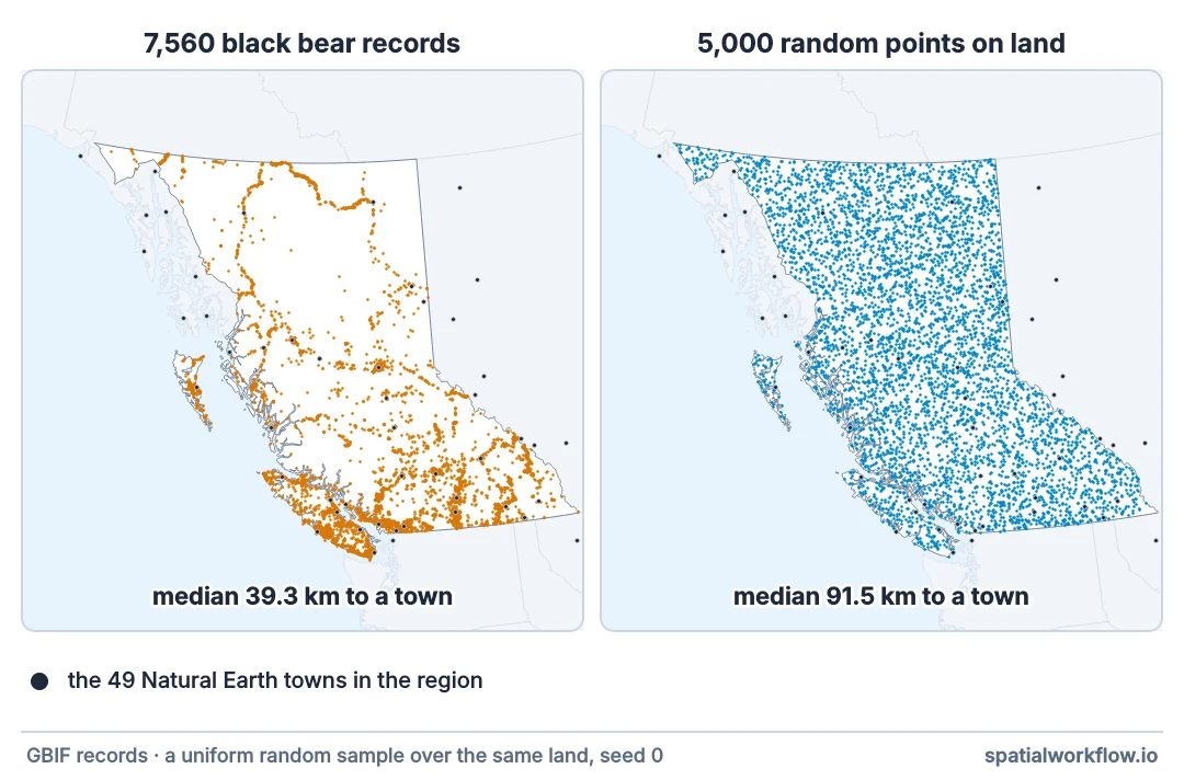
A map of occurrence records is a map of two things multiplied together: where the species is, and where people looked. The second one usually dominates. Records cluster along roads, around towns, inside parks with car parks, in the months when the weather is pleasant, and on Saturdays.
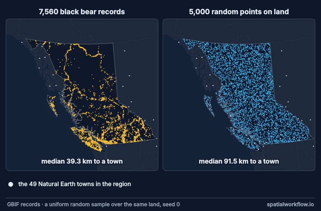
The effect is not subtle. Black bear records in British Columbia sit a median of 39 km from the nearest town; random points on the same land sit 92 km away. Within ten kilometres of a town, records are over-represented elevenfold.
Quick answer
Compare the records against a null sample of the same area:
import io, os, zipfile
import numpy as np, pandas as pd, geopandas as gpd, requests
from shapely import STRtree
from gbif import search

def natural_earth(name, url):
    """Download a Natural Earth layer once and keep it."""
    path = f"bio/{name}.gpkg"
    if not os.path.exists(path):
        blob = requests.get(url, timeout=300).content
        zipfile.ZipFile(io.BytesIO(blob)).extractall(f"bio/{name}")
        shp = [f for f in os.listdir(f"bio/{name}") if f.endswith(".shp")][0]
        gpd.read_file(f"bio/{name}/{shp}").to_file(path, driver="GPKG")
    return gpd.read_file(path)

NE = "https://naciscdn.org/naturalearth/10m/cultural"
region = natural_earth("ne_states", f"{NE}/ne_10m_admin_1_states_provinces.zip")
region = region.query("name == 'British Columbia'").to_crs(3005)
towns = natural_earth("ne_places", f"{NE}/ne_10m_populated_places.zip").cx[-140:-114, 48:60]
towns = towns.to_crs(3005)

bears = search(taxonKey=2433407, country="CA", stateProvince="British Columbia",
               hasCoordinate="true")
records = gpd.GeoDataFrame(bears, crs=4326,
                           geometry=gpd.points_from_xy(bears.decimalLongitude,
                                                       bears.decimalLatitude)).to_crs(3005)

rng = np.random.default_rng(0)
minx, miny, maxx, maxy = region.total_bounds
land = region.union_all()
sample = []
while len(sample) < 5_000:                                  # a null: uniform over the land
    cand = gpd.GeoSeries(gpd.points_from_xy(rng.uniform(minx, maxx, 4000),
                                            rng.uniform(miny, maxy, 4000)), crs=3005)
    sample += list(cand[cand.within(land)])
null = gpd.GeoSeries(sample[:5_000], crs=3005)

tree = STRtree(towns.geometry.values)
def km_to_town(points):
    idx = tree.nearest(points.values)
    return points.distance(gpd.GeoSeries(towns.geometry.values[idx], crs=3005),
                           align=False) / 1000

observed, expected = km_to_town(records.geometry), km_to_town(null)
print(f"{len(records):,} records, {len(towns)} towns, {len(null):,} null points")
print(f"median distance to a town: records {observed.median():.1f} km, "
      f"random land {expected.median():.1f} km")
for cut in (10, 25, 50):
    o, e = (observed < cut).mean(), (expected < cut).mean()
    print(f"  within {cut:>2} km: records {o:.1%}, land {e:.1%}, "
          f"over-represented {o / e:.1f}×")
7,560 records, 49 towns, 5,000 null points
median distance to a town: records 39.2 km, random land 91.5 km
within 10 km: records 11.7%, land 1.0%, over-represented 11.7×
within 25 km: records 32.7%, land 5.3%, over-represented 6.2×
within 50 km: records 59.0%, land 19.7%, over-represented 3.0×
Without the null sample there is nothing to compare against, and a clustered map looks like a species that likes towns.
Name the bias, build a matching null, compare ratios
1. Name the bias you are testing for
Access, effort, season, day of week, observer skill, platform. Each has a different null and a different remedy.
2. Build a null of the same shape
Random points over the study area for spatial access bias; the calendar for temporal bias; the records of a related group for taxonomic bias.
3. Measure the ratio, not the count
"11% of records are within 10 km of a town" means nothing alone. "11% against 1% of the land" is the finding.
4. Use a target group as a better null
Records of similar, similarly-recorded species share the observer effort. Where they exist, they are a much better background than uniform random points.
5. Correct rather than ignore
Spatial thinning, target-group background samples, effort offsets in a model, or coarser grain. All of them lose information; ignoring the bias loses correctness.
6. Report the residual bias
No correction removes it. State what was corrected and what was not.
Weekend and seasonal effects in GBIF records
The data used on this page
Records come from the GBIF API via gbif.search, the paging function from the download guide plus eventDate and countryCode. Climate is WorldClim 2.1 bioclim at 10′ in bio/wc/; pa.protected_areas() is British Columbia's protected-area layer (EPSG:3005). GBIF changes daily, so the setup answers each request with the reply it got on 9 October 2026.
import hashlib
import io
import os
import zipfile

import requests

# GBIF adds and revises records daily. So that the numbers below reproduce, every GBIF request on
# this page is answered from the reply it got on 9 October 2026 (one file per request, named by a
# SHA-1 of its URL); any other request, or all of them once these lines are deleted, goes live.
SAVED = zipfile.ZipFile(io.BytesIO(requests.get(
    "https://data.spatialworkflow.io/gbif-api-2026-10-09.zip", timeout=300).content))
live_get = requests.get


def saved_get(url, params=None, **kwargs):
    prepared = requests.Request("GET", url, params=params).prepare()
    try:
        body = SAVED.read(hashlib.sha1(prepared.url.encode()).hexdigest()[:16] + ".json")
    except KeyError:
        return live_get(url, params=params, **kwargs)
    reply = requests.models.Response()
    reply.status_code, reply._content, reply.url = 200, body, prepared.url
    reply.headers["Content-Type"] = "application/json"
    return reply


requests.get = saved_get

os.makedirs("bio/wc", exist_ok=True)
with open("gbif.py", "w") as f:
    f.write('''
import pandas as pd, requests

API = "https://api.gbif.org/v1"
MAX_OFFSET = 100_000
FIELDS = ["key", "species", "speciesKey", "decimalLongitude", "decimalLatitude",
          "coordinateUncertaintyInMeters", "year", "month", "basisOfRecord",
          "datasetKey", "institutionCode", "issues", "eventDate", "countryCode"]


def count(**params):
    return requests.get(f"{API}/occurrence/search", params={**params, "limit": 0}, timeout=120).json()["count"]


def search(limit=None, page=300, **params):
    total = count(**params)
    if limit is None and total > MAX_OFFSET:
        raise ValueError(f"{total:,} records exceeds the {MAX_OFFSET:,} offset limit")
    rows, offset = [], 0
    target = total if limit is None else min(limit, total)
    while offset < target:
        body = requests.get(f"{API}/occurrence/search",
                            params={**params, "limit": min(page, target - offset), "offset": offset},
                            timeout=180).json()
        rows += body["results"]
        offset += len(body["results"])
        if body["endOfRecords"] or not body["results"]:
            break
    return pd.DataFrame([{f: r.get(f) for f in FIELDS} for r in rows])
''')
with open("pa.py", "w") as f:
    f.write('''
import os
import geopandas as gpd

URL = ("https://services6.arcgis.com/ubm4tcTYICKBpist/arcgis/rest/services/"
       "British_Columbia_Parks_Ecological_Reserves_and_Protected_Areas/FeatureServer/0/query"
       "?where=1%3D1&outFields=PROTECTED_LANDS_NAME&outSR=3005&f=geojson")


def protected_areas():
    if not os.path.exists("bio/bc_protected.gpkg"):
        gpd.read_file(URL).to_file("bio/bc_protected.gpkg")
    return gpd.read_file("bio/bc_protected.gpkg")
''')
if not os.path.exists("bio/wc/wc2.1_10m_bio_1.tif"):
    blob = requests.get("https://geodata.ucdavis.edu/climate/worldclim/2_1/base/wc2.1_10m_bio.zip", timeout=600).content
    zipfile.ZipFile(io.BytesIO(blob)).extractall("bio/wc")
print(len([n for n in os.listdir("bio/wc") if n.endswith(".tif")]), "WorldClim layers")
19 WorldClim layers
Example 1 — the weekend effect
dates = pd.to_datetime(records.eventDate, errors="coerce", utc=True)
dated = dates.notna()
print(f"{dated.sum():,} of {len(records):,} records carry a parsable date")

by_day = dates[dated].dt.dayofweek.value_counts().sort_index()
names = ["Mon", "Tue", "Wed", "Thu", "Fri", "Sat", "Sun"]
for i, n in by_day.items():
    bar = "█" * int(40 * n / by_day.max())
    print(f"  {names[int(i)]}  {n:>5,}  {bar}")
weekend = (dates[dated].dt.dayofweek >= 5).mean()
print(f"\nweekend share: {weekend:.1%} against {2 / 7:.1%} of days "
      f"({weekend / (2 / 7):.2f}× )")
3,539 of 7,560 records carry a parsable date
Mon 476 █████████████████████████████████
Tue 458 ████████████████████████████████
Wed 497 ███████████████████████████████████
Thu 491 ██████████████████████████████████
Fri 493 ██████████████████████████████████
Sat 566 ████████████████████████████████████████
Sun 558 ███████████████████████████████████████
weekend share: 31.8% against 28.6% of days (1.11× )
Example 2 — the season, which is both bias and biology
by_month = dates[dated].dt.month.value_counts().sort_index()
for m, n in by_month.items():
    bar = "█" * int(40 * n / by_month.max())
    print(f"  {int(m):>2}  {n:>5,}  {bar}")
peak, trough = by_month.idxmax(), by_month.idxmin()
print(f"\npeak month {int(peak)} with {by_month.max():,} records; "
      f"quietest {int(trough)} with {by_month.min():,}")
print(f"ratio {by_month.max() / by_month.min():.0f}:1")
print("black bears hibernate, and people hike in summer — "
      "this curve is both effects and cannot separate them")
1 15
2 10
3 39 ██
4 186 ██████████
5 615 ██████████████████████████████████
6 711 ████████████████████████████████████████
7 582 ████████████████████████████████
8 542 ██████████████████████████████
9 529 █████████████████████████████
10 229 ████████████
11 64 ███
12 17
peak month 6 with 711 records; quietest 2 with 10
ratio 71:1
black bears hibernate, and people hike in summer — this curve is both effects and cannot separate them
Example 3 — what a target-group background changes
coyote = search(taxonKey=5219153, country="CA", stateProvince="British Columbia",
                hasCoordinate="true")                       # recorded by the same people
target = gpd.GeoDataFrame(coyote, crs=4326,
                          geometry=gpd.points_from_xy(coyote.decimalLongitude,
                                                      coyote.decimalLatitude)).to_crs(3005)
target_d = km_to_town(target.geometry)

print(f"{'sample':<28}{'n':>8}{'median km':>12}{'within 10 km':>14}")
for name, n, d in [("black bear records", len(records), observed),
                   ("coyote records", len(target), target_d),
                   ("uniform random land", len(null), expected)]:
    print(f"{name:<28}{n:>8,}{d.median():>12.1f}{(d < 10).mean():>13.1%}")

print(f"\nbear vs uniform land, within 10 km: "
      f"{(observed < 10).mean() / (expected < 10).mean():.1f}× over-represented")
print(f"bear vs another recorded mammal:    "
      f"{(observed < 10).mean() / (target_d < 10).mean():.2f}×")
sample n median km within 10 km
black bear records 7,560 39.2 11.7%
coyote records 2,545 17.1 34.6%
uniform random land 5,000 91.5 1.0%
bear vs uniform land, within 10 km: 11.7× over-represented
bear vs another recorded mammal: 0.34×
Against uniform land the bears look enormously biased towards towns. Against another mammal recorded by the same people, they look like the species that is furthest from towns of the two — the ratio flips from elevenfold over-represented to a third of the target group's rate. The uniform null measures access bias plus habitat plus everything else and blames it all on bias; the target group measures only what distinguishes this species from the others, which is what a distribution model should be fitting.
Why target-group backgrounds work
Why uniform random points are the wrong null on their own
Uniform points assume that every square kilometre was equally likely to be searched, which is false everywhere. The ratio against a uniform null measures access bias plus habitat preference plus everything else at once, and attributing the whole of it to bias over-corrects.
Why the target-group background works
If you sample background points from the occurrence records of a group recorded by the same methods, the background carries the same access bias as the presences. What remains after the comparison is the part of the pattern that distinguishes this species from the others — which is the quantity a distribution model should be fitting.
Why the temporal biases are worth checking even so
A weekend effect tells you the records are recreational; a summer peak on a hibernating species tells you the seasonality is unusable without correction. Neither changes a spatial model much, and both change how the record set should be described, which is what a reader needs to judge it.
Roads, protected areas and taxonomic bias
- Roads are a better access proxy than towns where a road layer exists; distance-to-road is the classic covariate.
- Protected areas attract recording effort, which makes "more species in parks" partly an artefact.
- eBird publishes checklists with effort — duration, distance, complete-checklist flags — which is far better than presence-only.
- Museum collections are biased towards expedition routes and institution neighbourhoods, in a different pattern from citizen science.
- Taxonomic bias: birds and butterflies are recorded orders of magnitude more than beetles.
- Correcting twice — thinning and a target-group background and an effort offset — can over-correct; test one at a time.
Internal links
- Species occurrence data explained — what a record is
- How to thin occurrence records spatially — the usual spatial correction
- A richness map is a map of sampling effort — the fix guide
- Species distribution models explained — where the background sample goes
- How to build a species richness grid — where bias becomes visible
- Sample design explained: where to measure — what unbiased sampling would look like
FAQ
Why do occurrence records cluster near roads and towns?
Because that is where people are. Records are a sample of observer effort as much as of the species.
How do I tell bias from real habitat preference?
Compare the records with a null sample of the same area, and preferably with a target group recorded by the same methods.
What is a target-group background?
Background points drawn from the records of similar species, so the background carries the same sampling bias as the presences.
Does thinning fix it?
It reduces the clustering, not the underlying access bias. It is a partial correction, and it costs records.
Is a weekend effect a problem?
For a spatial model, rarely. For anything about timing or effort, it tells you what kind of data you have.
Can bias be removed?
No. It can be measured, partly corrected, and reported.