
How to build a species richness grid
On this page
Problem statement
Species richness per grid cell is the standard first map in any biodiversity analysis, and it is usually built by downloading every record in the region and counting distinct species per cell. For British Columbia's mammals that is 133,305 records of 174 species — and the download is the slow, fragile part of a calculation whose answer is one short number per cell.
GBIF will do the counting server-side. A faceted query returns the record count and the species list for any polygon in a fraction of a second, which turns a grid of cells into a grid of small, independent queries.
Quick answer
One query per cell, faceted on species:
import time
import numpy as np, pandas as pd, requests

API = "https://api.gbif.org/v1/occurrence/search"

def cell_counts(west, south, east, north, pause=0.2, **params):
    """Record count and species list for one cell, counted by GBIF.

    A grid is hundreds of requests, so this backs off on HTTP 429 rather than
    parsing the rate-limit message as if it were a result.
    """
    wkt = (f"POLYGON(({west} {south},{east} {south},{east} {north},"
           f"{west} {north},{west} {south}))")
    for attempt in range(6):
        r = requests.get(API, params={**params, "geometry": wkt, "hasCoordinate": "true",
                                      "facet": "speciesKey", "facetLimit": 1000,
                                      "limit": 0}, timeout=180)
        if r.status_code == 429:
            time.sleep(2 ** attempt)
            continue
        r.raise_for_status()
        body = r.json()
        time.sleep(pause)
        facets = body.get("facets") or [{}]
        return body["count"], facets[0].get("counts", [])
    raise RuntimeError("rate limited six times in a row")

records, species = cell_counts(-123.5, 49.0, -122.5, 49.5, taxonKey=359)
print(f"one 0.5° cell near Vancouver: {records:,} mammal records, "
      f"{len(species)} species")
print("commonest:", [(s["name"], s["count"]) for s in species[:3]])
one 0.5° cell near Vancouver: 26,660 mammal records, 95 species
commonest: [('5219681', 4310), ('2434793', 2754), ('2437281', 2147)]
The counting happens in GBIF's index. Nothing is downloaded, and the cell is defined by a polygon rather than by post-hoc binning, which means the grid can be whatever shape the question needs.
Grain first, equal-area cells, server-side counts
1. Choose the grain before you look at the data
Cell size is the single biggest control on a richness map. Choose it from the question and the coordinate uncertainty, not from how the map looks.
2. Use an equal-area grid where the latitude range is wide
A 0.5° cell at 49°N covers about 2,000 km²; at 60°N, about 1,500 km². A degree grid makes northern cells look species-poor partly because they are smaller.
3. Query the count and the species list together
The facet gives both. Keeping the record count is what makes the effort correction in the next guide possible.
4. Cache, pause, and handle the rate limit
A grid is hundreds of requests. GBIF answers too many with HTTP 429 and a body that is a JSON list, so code that goes straight to .json()["count"] crashes with a confusing type error instead of backing off.
5. Check the facet limit
facetLimit caps how many species come back. If a cell returns exactly the limit, the richness is truncated and the map is wrong in the richest cells.
6. Map richness and effort side by side
They correlate strongly nearly everywhere. Publishing one without the other invites the reader to interpret sampling as biology.
A richness grid over British Columbia
The data used on this page
Every number below comes from GBIF's API. GBIF adds and revises records daily, so the setup answers each GBIF request this page makes from the reply it got on 9 October 2026, and lets any other request through live.
import hashlib, io, zipfile

import requests

# GBIF adds and revises records daily. So that the numbers below reproduce, every GBIF request on
# this page is answered from the reply it got on 9 October 2026 (one file per request, named by a
# SHA-1 of its URL); any other request, or all of them once these lines are deleted, goes live.
SAVED = zipfile.ZipFile(io.BytesIO(requests.get(
    "https://data.spatialworkflow.io/gbif-api-2026-10-09.zip", timeout=300).content))
live_get = requests.get


def saved_get(url, params=None, **kwargs):
    prepared = requests.Request("GET", url, params=params).prepare()
    try:
        body = SAVED.read(hashlib.sha1(prepared.url.encode()).hexdigest()[:16] + ".json")
    except KeyError:
        return live_get(url, params=params, **kwargs)
    reply = requests.models.Response()
    reply.status_code, reply._content, reply.url = 200, body, prepared.url
    reply.headers["Content-Type"] = "application/json"
    return reply


requests.get = saved_get
Example 1 — a grid over the province
WEST, EAST, SOUTH, NORTH = -139.0, -114.0, 48.0, 60.0
STEP = 1.0

grid = []
for west in np.arange(WEST, EAST, STEP):
    for south in np.arange(SOUTH, NORTH, STEP):
        n, sp = cell_counts(round(west, 3), round(south, 3),
                            round(west + STEP, 3), round(south + STEP, 3),
                            taxonKey=359, country="CA")
        grid.append({"west": west, "south": south, "records": n,
                     "richness": len(sp), "truncated": len(sp) >= 1000})
cells = pd.DataFrame(grid)

occupied = cells[cells.records > 0]
print(f"{len(cells)} cells, {len(occupied)} with any records")
print(f"records: total {cells.records.sum():,}, median per occupied cell "
      f"{occupied.records.median():,.0f}, max {cells.records.max():,}")
print(f"richness: median {occupied.richness.median():.0f}, max {cells.richness.max()}, "
      f"cells at the facet limit: {cells.truncated.sum()}")
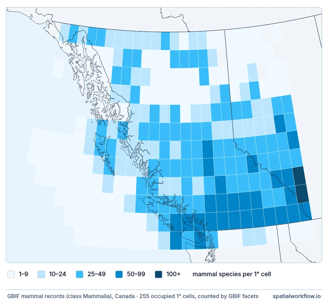
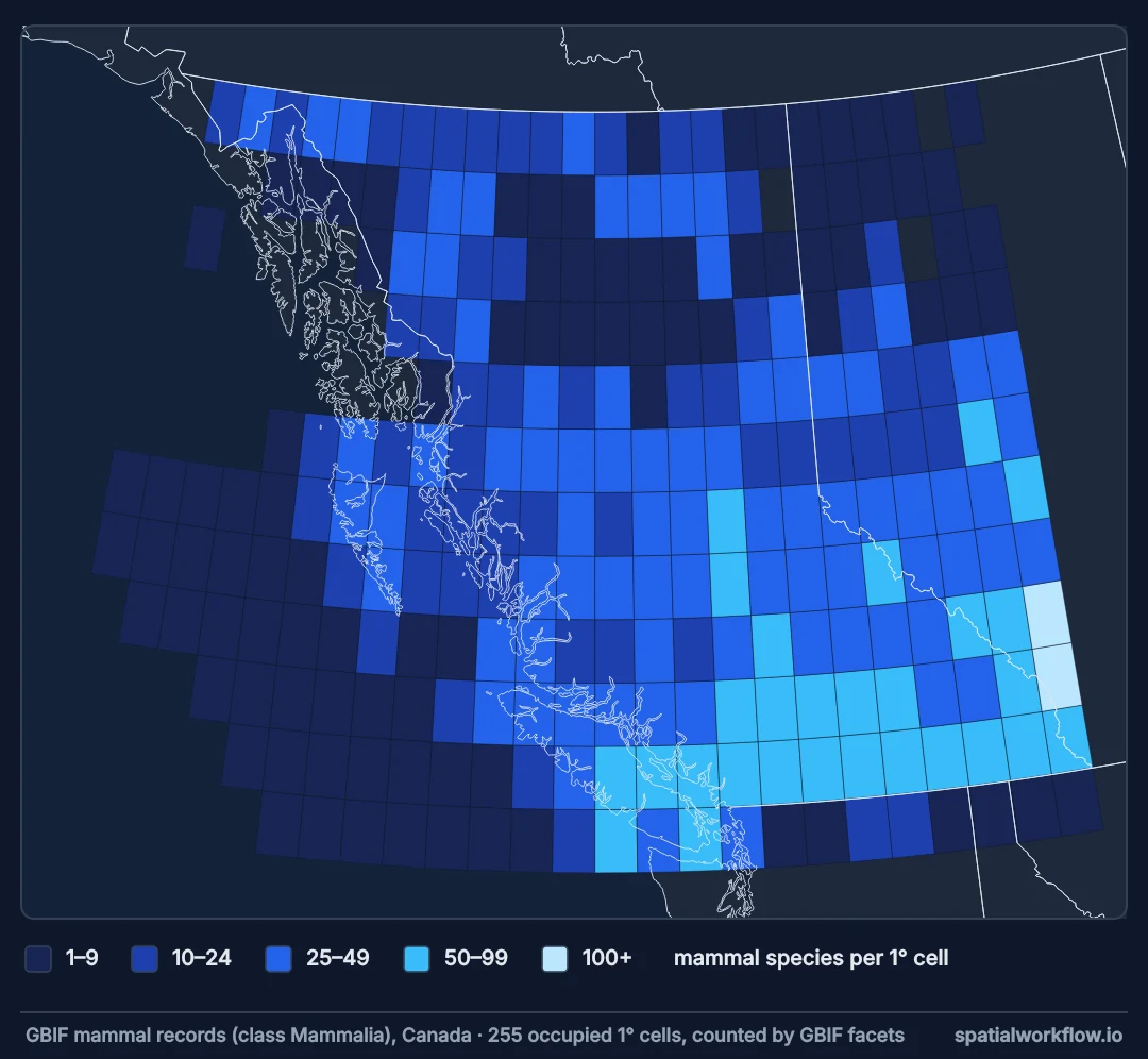
300 cells, 255 with any records
records: total 224,094, median per occupied cell 102, max 32,622
richness: median 19, max 162, cells at the facet limit: 0
Example 2 — richness against effort
from scipy import stats

busy = occupied[occupied.records >= 10]
r = stats.spearmanr(np.log10(busy.records), busy.richness)
print(f"{len(busy)} cells with 10+ records")
print(f"Spearman correlation between log(records) and richness: "
      f"{r.statistic:.2f} (p = {r.pvalue:.1e})")

bins = [10, 100, 1_000, 10_000, 1_000_000]
print(f"\n{'records in cell':<22}{'cells':>7}{'median richness':>18}")
for lo, hi in zip(bins[:-1], bins[1:]):
    sel = busy[(busy.records >= lo) & (busy.records < hi)]
    if len(sel):
        print(f"{f'{lo:,}–{hi:,}':<22}{len(sel):>7}{sel.richness.median():>18.0f}")
221 cells with 10+ records
Spearman correlation between log(records) and richness: 0.93 (p = 5.0e-98)
records in cell cells median richness
10–100 93 8
100–1,000 92 32
1,000–10,000 32 56
10,000–1,000,000 4 88
A Spearman correlation of 0.93 between effort and richness is the normal state of occurrence data. It does not mean the richness map is worthless; it means the map cannot be read as biology without the effort map beside it.
Example 3 — what the grain does
for step in (0.5, 1.0, 2.0):
    sample = []
    for west in np.arange(-126.0, -120.0, step):
        for south in np.arange(49.0, 53.0, step):
            n, sp = cell_counts(round(west, 3), round(south, 3),
                                round(west + step, 3), round(south + step, 3),
                                taxonKey=359, country="CA")
            if n:
                sample.append(len(sp))
    print(f"{step}° cells: {len(sample):>3} occupied, "
          f"median richness {np.median(sample):>5.1f}, max {max(sample):>3}")
0.5° cells: 95 occupied, median richness 25.0, max 89
1.0° cells: 24 occupied, median richness 49.0, max 94
2.0° cells: 6 occupied, median richness 78.0, max 115
Doubling the cell size doubles the median richness at the first step and adds 60% at the second — a bigger cell samples more habitat and more effort. Any statement of the form "this region has N species per cell" is a statement about the grid as much as about the fauna.
Example 4 — the province totals quoted at the top
province = requests.get(API, params={"taxonKey": 359, "country": "CA", "stateProvince": "British Columbia",
                                     "hasCoordinate": "true", "limit": 0,
                                     "facet": "speciesKey", "facetLimit": 1000}, timeout=180).json()
print(f"British Columbia mammals: {province['count']:,} records, "
      f"{len(province['facets'][0]['counts'])} species")
British Columbia mammals: 133,305 records, 174 species
Server-side counts and facet limits
Why the server-side count is the right default
Richness is an aggregate, and aggregates should be computed where the data is. The faceted query is one HTTP round trip per cell against an index built for exactly this; the download-and-bin route moves hundreds of thousands of records so that a laptop can do a groupby. The download is still necessary when the question needs the individual records — dates, datasets, uncertainty — and unnecessary when it does not.
Why the facet limit matters
facetLimit is how many distinct species the API will return for a cell. A cell that returns exactly that number has been truncated, and its richness is a lower bound. Checking for it costs one comparison and catches a silent, systematic error in precisely the cells a richness map is about.
Why richness per cell is not richness
The number of species recorded in a cell depends on the cell's size, the effort spent in it, and the detectability of the species there — in roughly that order, before any ecology. The next guide corrects for the second of those; the first is a choice, and the third needs survey data this kind of record cannot provide.
Winding order, the dateline and hexagons
- Winding order: GBIF wants counter-clockwise WKT polygons; a clockwise one is read as the rest of the planet.
- Dateline and poles: split cells that cross 180°, and expect degree cells to be tiny near the poles.
countryplusgeometryis an intersection, which is what keeps coastal cells from picking up the neighbouring jurisdiction.- Hexagons (H3, ISEA) avoid the latitude problem entirely and are worth the extra code for a continental map.
- Occurrence status: absence records are in the index; filter them out or the richness includes species recorded as not present.
- The GBIF map API serves pre-aggregated tiles if all you need is a picture.
Internal links
- Biodiversity metrics explained — what richness does and does not measure
- How to correct richness for sampling effort — the next step
- A richness map is a map of sampling effort — the fix guide
- Sampling bias in occurrence data explained — why effort varies
- How to download GBIF occurrences in Python — when you do need the records
- How to aggregate points into H3 hexagons and map them — an equal-area alternative
FAQ
How do I count species per grid cell?
Query GBIF per cell with a polygon and a speciesKey facet; the facet length is the richness and the count is the effort.
Do I have to download the records first?
No, and usually you should not. Download only when the analysis needs individual records.
What cell size should I use?
One chosen from the question and the coordinate uncertainty. Richness per cell rises with cell size, so the grain is part of the answer.
Why is my richness capped at a round number?
The facet limit truncated it. Raise facetLimit and check whether any cell still hits it.
Should I use degrees or an equal-area grid?
Equal-area for anything spanning a wide latitude range; degree cells shrink towards the poles.
Why does richness track record count so closely?
Because more effort finds more species. That correlation is the reason richness maps need an effort correction.