How to Compare CAMS Air Quality with Monitoring Stations in Python

On this page

Problem statement

The Copernicus Atmosphere Monitoring Service publishes hourly air quality for all of Europe at about 10 km, free, back several years and into the next few days. It is the obvious way to fill the gaps between monitoring stations — and the obvious question is how good it is where there are stations to check it against.

The answer depends on what the station measures. A 10 km model cell is a neighbourhood average; a background station is a neighbourhood sample; a kerbside station is a street. Evaluating the model against all stations together mixes a fair test with an unfair one, and the resulting statistics describe neither.

Quick answer

Fetch the model at each station's coordinates, align the hours, and compute bias, error and correlation separately by station type:

import io, requests, numpy as np, pandas as pd

API = "https://eeadmz1-downloads-api-appservice.azurewebsites.net/ParquetFile/urls"
META = "https://discomap.eea.europa.eu/map/fme/metadata/PanEuropean_metadata.csv"
r = requests.post(API, json={"countries": ["DE"], "cities": ["Berlin"], "pollutants": ["NO2"],
                             "dataset": 2, "dateTimeStart": "2023-01-01T00:00:00Z",
                             "dateTimeEnd": "2023-12-31T23:00:00Z", "aggregationType": "hour"},
                  timeout=120)
meta = pd.read_csv(META, sep="\t", low_memory=False,
                   storage_options={"User-Agent": "spatialworkflow-examples/1.0"}).drop_duplicates("SamplingPoint")   # EEA refuses Python's default agent
obs = {}
for url in [u.strip() for u in r.text.splitlines()[1:] if u.strip()]:
    d = pd.read_parquet(io.BytesIO(requests.get(url, timeout=120).content))
    d["Value"] = pd.to_numeric(d.Value, errors="coerce")
    y = d[(d.Start >= "2023-01-01") & (d.Start < "2024-01-01") & (d.Validity > 0)]
    if len(y) >= 0.9 * 8760:
        s = pd.Series(y.Value.to_numpy(), index=y.Start.dt.tz_localize("Etc/GMT-1").dt.tz_convert("UTC"))
        obs[d.Samplingpoint.iloc[0].split("/")[1]] = s
st = meta.set_index("SamplingPoint").loc[list(obs)]

j = requests.get("https://air-quality-api.open-meteo.com/v1/air-quality", params={
    "latitude": ",".join(f"{v:.4f}" for v in st.Latitude),
    "longitude": ",".join(f"{v:.4f}" for v in st.Longitude),
    "hourly": "nitrogen_dioxide", "start_date": "2023-01-01", "end_date": "2023-12-31",
    "domains": "cams_europe"}, timeout=300).json()
rows = []
for sp, res in zip(st.index, j):
    model = pd.Series(np.array(res["hourly"]["nitrogen_dioxide"], dtype=float),
                      index=pd.to_datetime(res["hourly"]["time"]).tz_localize("UTC"))
    both = pd.concat({"obs": obs[sp], "cams": model}, axis=1).dropna()
    rows.append({"point": sp[7:14], "type": st.loc[sp, "AirQualityStationType"],
                 "obs": both.obs.mean(), "cams": both.cams.mean(),
                 "bias": (both.cams - both.obs).mean(),
                 "rmse": np.sqrt(((both.cams - both.obs) ** 2).mean()),
                 "r": both.corr().iloc[0, 1]})
ev = pd.DataFrame(rows)
print(ev.groupby("type")[["obs", "cams", "bias", "rmse", "r"]].mean().round(2).to_string())

              obs   cams   bias   rmse     r
type                                        
background  11.48  11.10  -0.38   5.46  0.83
traffic     24.59  13.08 -11.51  15.53  0.68

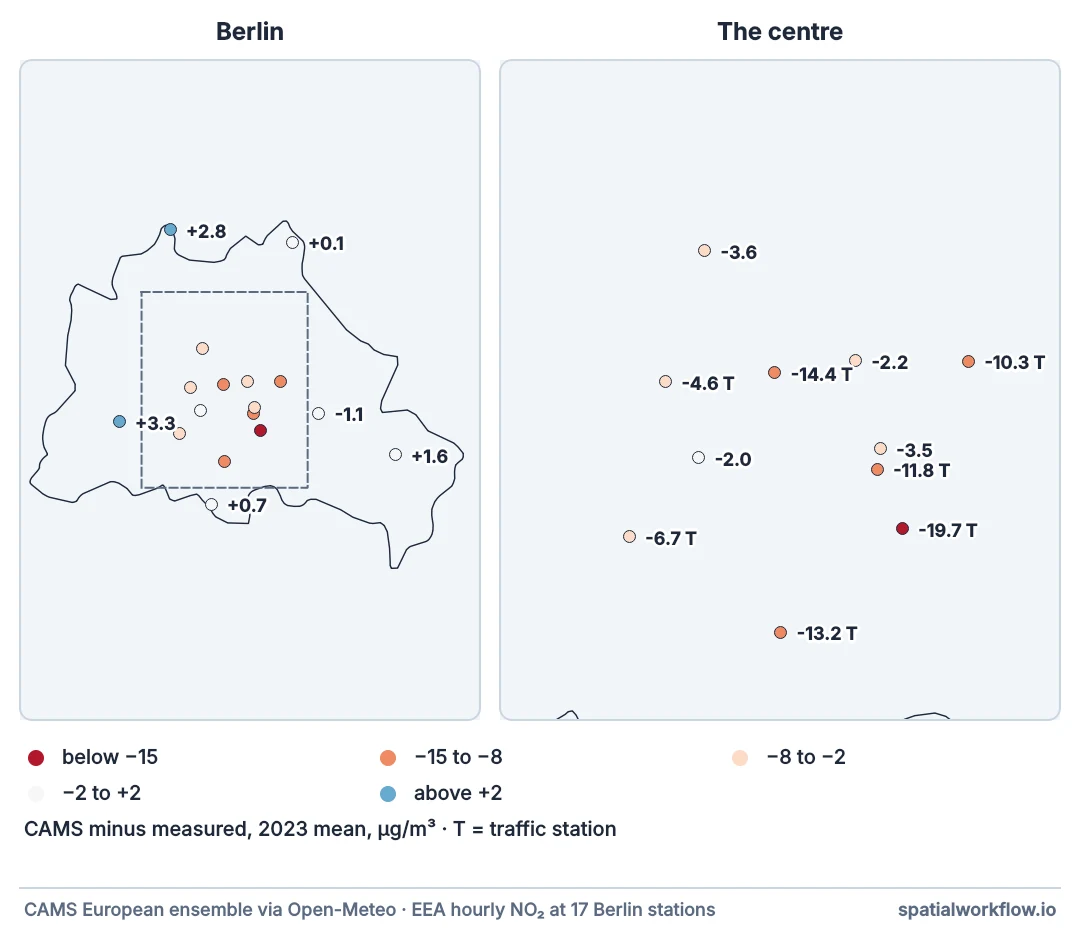
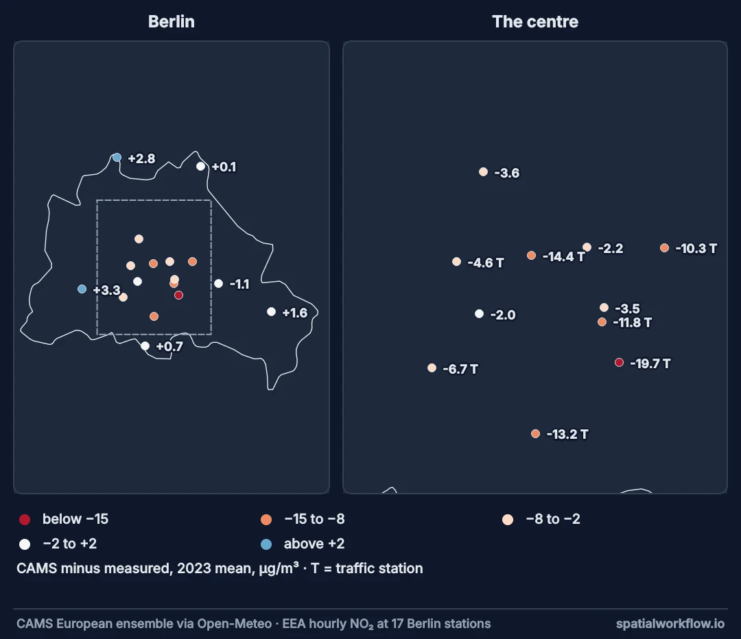
Against background stations the model is nearly unbiased over the year (−0.4 µg/m³) and well correlated hour by hour (r = 0.83). Against kerbside stations it is 11.5 µg/m³ low — roughly the traffic increment — not because the model is wrong, but because it is not trying to predict a kerb.

Two maps of Berlin’s monitoring stations coloured by the CAMS model’s bias: background stations near white, within a few micrograms, and traffic stations in the centre in orange and red, with the model 4.6 to 19.7 micrograms too low. — Each station coloured by CAMS minus measured over 2023, the centre enlarged on the right. At background stations the model is within about 4 µg/m³ either way. At every traffic station (T) it is too low, by 4.6 to 19.7 µg/m³: a 10 km model grid cannot see a kerbside, and the average −11.5 µg/m³ bias for traffic stations is that, not a model fault.

UTC series, like with like, several statistics, episodes

1. Get both series in UTC

Open-Meteo returns the model in UTC (or the zone you request). EEA observations are in the country's standard time — UTC+1 for Germany, all year. A one-hour offset misaligns every hour of the comparison.

2. Compare like with like

Evaluate the model against the station type it represents: urban and rural background. Report kerbside results separately, as a measure of what the model's resolution misses.

3. Use several statistics

Mean bias (is it systematically high or low?), RMSE (how big are the errors?), correlation (does it get the timing right?). A model can have zero bias and poor correlation, or good correlation and a large bias.

4. Look at the diurnal cycle

Models often reproduce daily means better than hours. Comparing mean profiles by hour shows whether the model's emissions timing and mixing-layer evolution match reality.

5. Check episodes, not just averages

The days that matter are the high ones. Compare the model on the observed top-decile days: many models underpredict peaks.

Nearly unbiased against the stations it represents, far low against the kerbs.

Station-by-station, diurnal and worst-day comparisons

Example 1 — station by station

print(ev.sort_values("obs").round(1).to_string(index=False))

  point       type  obs  cams  bias  rmse   r
DEBE062 background  6.7   9.5   2.8   4.9 0.8
DEBE056 background  7.5   9.1   1.6   3.4 0.9
DEBE032 background  7.6  10.9   3.3   5.8 0.8
DEBE027 background  8.3   9.0   0.7   4.1 0.8
DEBE051 background  8.8   8.9   0.1   3.9 0.8
DEBE066 background 12.1  11.0  -1.1   5.2 0.8
DEBE018 background 15.0  13.0  -2.0   6.1 0.9
DEBE034 background 15.6  12.1  -3.5   7.2 0.8
DEBE068 background 15.7  13.5  -2.2   6.6 0.8
DEBE010 background 17.5  13.9  -3.6   7.3 0.8
DEBE067    traffic 18.5  14.0  -4.6   8.0 0.8
DEBE061    traffic 19.6  12.9  -6.7  11.0 0.8
DEBE065    traffic 23.8  13.5 -10.3  14.1 0.7
DEBE126    traffic 23.9  12.1 -11.8  15.3 0.7
DEBE069    traffic 26.1  13.0 -13.2  17.6 0.6
DEBE125    traffic 28.4  13.9 -14.4  18.2 0.6
DEBE063    traffic 31.8  12.1 -19.7  24.5 0.5

Across the background stations the model spans 8.9–13.9 µg/m³ where the observations span 6.7–17.5: it overpredicts the city edge and underpredicts the inner districts, because a 10 km cell blends both. At the kerbs the error grows with the traffic, to −19.7 µg/m³ at the busiest.

Example 2 — the diurnal cycle

bg_points = ev.loc[ev.type == "background", "point"]
profile = []
for sp, res in zip(st.index, j):
    if sp[7:14] not in set(bg_points):
        continue
    model = pd.Series(np.array(res["hourly"]["nitrogen_dioxide"], dtype=float),
                      index=pd.to_datetime(res["hourly"]["time"]).tz_localize("UTC"))
    both = pd.concat({"obs": obs[sp], "cams": model}, axis=1).dropna()
    local = both.tz_convert("Europe/Berlin")
    profile.append(local.groupby(local.index.hour).mean())
prof = sum(profile) / len(profile)
print(prof.loc[[2, 6, 8, 12, 16, 19, 22]].round(1).to_string())
print(f"\nobserved peak {prof.obs.idxmax():02d}:00, model peak {prof.cams.idxmax():02d}:00")

     obs  cams
2   10.7  10.8
6   13.6  10.6
8   14.9  14.0
12   8.5   8.9
16   9.6   8.9
19  12.6  12.3
22  13.6  13.5

observed peak 07:00, model peak 08:00

The model reproduces the evening and night closely and misses the morning rush — 10.6 against 13.6 µg/m³ at 06:00, peaking an hour late. The daily shape is where a model reveals its assumptions about emission timing and the evolution of the mixing layer. Differences here matter for anything that uses hourly model values — exposure during commuting, for example.

Example 3 — the worst days

daily = []
for sp, res in zip(st.index, j):
    if sp[7:14] not in set(bg_points):
        continue
    model = pd.Series(np.array(res["hourly"]["nitrogen_dioxide"], dtype=float),
                      index=pd.to_datetime(res["hourly"]["time"]).tz_localize("UTC"))
    daily.append(pd.concat({"obs": obs[sp], "cams": model}, axis=1).dropna().resample("D").mean())
days = pd.concat(daily).groupby(level=0).mean()
top = days[days.obs >= days.obs.quantile(0.9)]
print(f"all days:        observed {days.obs.mean():.1f}, model {days.cams.mean():.1f} µg/m³")
print(f"top-decile days: observed {top.obs.mean():.1f}, model {top.cams.mean():.1f} µg/m³ "
      f"({top.cams.mean() / top.obs.mean() - 1:+.0%})")
print(f"daily correlation: {days.corr().iloc[0, 1]:.2f}")

all days:        observed 11.5, model 11.1 µg/m³
top-decile days: observed 23.6, model 23.2 µg/m³ (-2%)
daily correlation: 0.99

A daily correlation of 0.99 with the background mean, and top-decile days within 2%, is better than an independent 10 km model should manage. The reason is that it is not independent: the CAMS European system assimilates surface observations — from networks including these — into the initial state of each forecast, so the model carries the stations' imprint. Treat this agreement as an upper bound on how well the model does away from monitored sites, and for an honest test withhold stations the system does not assimilate, or compare with longer-range forecasts. In general, averages can look excellent while episodes are underpredicted; report episode statistics alongside annual ones.

The daily cycle is where timing assumptions show.

A ten-kilometre cell cannot match a kerb

Why the model cannot match a kerb

A 10 km cell averages every street, park and lake in 100 km². The traffic increment at a kerbside station is concentrated within tens of metres of one road; averaged over the cell, it nearly disappears. The model is right about the cell and wrong about the kerb, and both statements are true at once.

Why correlation and bias tell different stories

Correlation measures whether the model gets the ups and downs — the weather-driven variation — right. Bias measures whether its level is right. Weather is shared across a city, so a model driven by good meteorology correlates well even where its level is off. Both need reporting.

Why episodes are harder

High-pollution episodes combine stagnant meteorology with local accumulation. Small errors in the mixing-layer height or wind, harmless on ordinary days, matter most in exactly those conditions, and coarse emission inventories miss local peaks.

Too high at the edge, too low in the centre, far too low at the kerb.

Domains, forecasts and representativeness

CAMS domains: cams_europe is the regional ensemble at about 0.1°; cams_global is much coarser.
Forecast vs reanalysis: the archive served through Open-Meteo is analysis/forecast data, not a reprocessed reanalysis; its versions change over time.
Units: CAMS NO2 is in µg/m³, matching European station data; check before comparing with ppb sources.
Station representativeness: suburban and rural-near-city stations sit in cells that also contain dense districts; some bias there is spatial, not model error.
Many stations: for a national evaluation, stratify by station type and area and report distributions, not only means.

Internal links

How to interpolate air quality station data — where the model beat interpolation
Air quality monitoring networks explained — what each station type represents
Air pollution meteorology explained — the weather the model has to get right
How to calculate population-weighted exposure — using the model field
How to download air quality station data in Python — the observation side
How to cross-validate an interpolation — evaluation statistics in general
How to compare air temperature with land surface temperature — stations against satellite

FAQ

How accurate is CAMS air quality data?

Against Berlin's background stations in 2023: bias −0.4 µg/m³, hourly r 0.83. Against kerbside stations it is biased low by the traffic increment. The analysis assimilates observations, so agreement at monitored sites overstates skill elsewhere.

Where can I get CAMS data in Python?

Through the Copernicus Atmosphere Data Store, or more simply through Open-Meteo's air quality API with domains=cams_europe.

Why is CAMS lower than my monitoring station?

If the station is kerbside, the 10 km model cannot resolve the road next to it.

What statistics should I report?

Mean bias, RMSE and correlation, by station type, plus performance on high-pollution days.

Do time zones matter for the comparison?

Yes. EEA data is in local standard time; model data is usually UTC. Align them before comparing hours.

Can CAMS replace monitoring stations?

It complements them. It fills space and time; stations anchor it and measure the local detail it cannot see.