How to Analyse Monthly Electricity Generation by Fuel in Python

Problem statement

Annual totals hide the shape of the electricity year. Demand peaks in summer for air conditioning and again in winter, solar follows the sun, wind blows hardest in spring, and something has to fill the gaps. EIA-923 holds the monthly net generation of every plant in twelve wide columns per measure, written in a way that makes a direct sum fail. This guide reshapes the 2025 file into monthly generation by source, measures each source's seasonal pattern and shows which one follows demand.

Quick answer

Take the twelve Netgen <Month> columns, replace EIA's "." placeholders with NaN, convert to float and sum by source. Transpose so months are rows, or melt to long format for plotting.

g = read_923()
months = [c for c in g.columns if c.startswith("Netgen ")]
g["source"] = g["MER Fuel Type Code"].map(MER).fillna("other")
mo = g[months].replace(".", np.nan).astype(float).groupby(g.source).sum().T / 1e6
mo.index = [c.split()[1][:3] for c in mo.index]
print(mo[["gas", "nuclear", "coal", "wind", "solar", "hydro"]].round(1).to_string())

source    gas  nuclear  coal  wind  solar  hydro
Jan     158.4     71.9  82.4  42.7   15.7   20.6
Feb     132.9     61.8  61.4  38.7   16.7   18.9
Mar     118.4     62.5  48.3  49.7   23.7   22.7
Apr     114.3     57.9  44.8  45.5   27.2   23.5
May     135.1     62.1  47.9  37.1   30.3   25.5
Jun     165.5     66.2  63.6  36.1   32.6   22.9
Jul     201.1     70.8  79.3  31.9   34.1   20.4
Aug     193.6     70.7  68.8  27.7   32.5   19.2
Sep     168.3     65.5  57.6  26.0   28.6   15.0
Oct     142.9     59.3  53.4  39.5   25.1   14.8
Nov     131.4     63.9  53.7  40.1   18.6   16.4
Dec     149.2     72.6  66.0  46.5   15.3   21.5

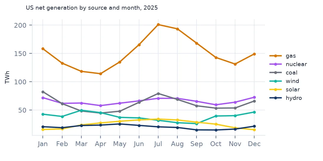
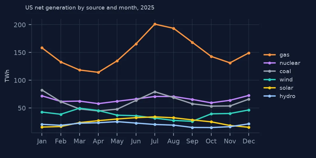
US generation in 2025 peaked in July: gas produced 201.1 TWh that month against 114.3 TWh in April. Solar ran from 15.3 TWh in December to 34.1 TWh in July; wind from 26.0 TWh in September to 49.7 TWh in March. Nuclear varied the least, between 57.9 and 72.6 TWh.

Reshaping and reading the months

1. Twelve columns per measure

print(f"{len(months)} net-generation columns; also {sum(c.startswith('Quantity ') for c in g.columns)} fuel-quantity and "
      f"{sum(c.startswith('Tot_MMBtu ') for c in g.columns)} heat-content columns")
long = g.melt(id_vars=["Plant Id", "source"], value_vars=months, var_name="month", value_name="MWh")
print(f"long format: {len(long):,} rows")

12 net-generation columns; also 12 fuel-quantity and 12 heat-content columns
long format: 226,668 rows

The file is wide: twelve columns for net generation, twelve for fuel quantity, twelve for heat content, and more. Melting the net-generation columns gives 226,668 rows of plant, source, month and MWh, the shape most plotting and grouping wants.

2. Shares through the year

sh = mo.div(mo.sum(axis=1), axis=0)
print("solar share by month:", sh.solar.round(3).to_dict())
print("wind share by month:", sh.wind.round(3).to_dict())

solar share by month: {'Jan': 0.039, 'Feb': 0.049, 'Mar': 0.071, 'Apr': 0.085, 'May': 0.088, 'Jun': 0.082, 'Jul': 0.076, 'Aug': 0.077, 'Sep': 0.078, 'Oct': 0.073, 'Nov': 0.056, 'Dec': 0.04}
wind share by month: {'Jan': 0.106, 'Feb': 0.114, 'Mar': 0.149, 'Apr': 0.142, 'May': 0.107, 'Jun': 0.091, 'Jul': 0.071, 'Aug': 0.066, 'Sep': 0.071, 'Oct': 0.115, 'Nov': 0.121, 'Dec': 0.122}

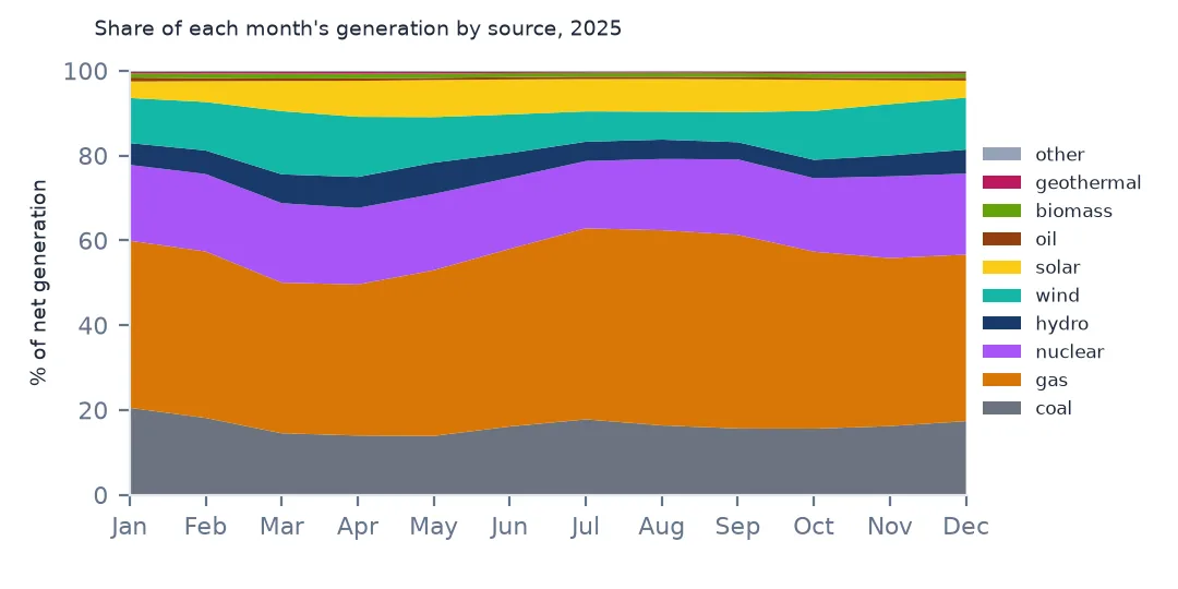
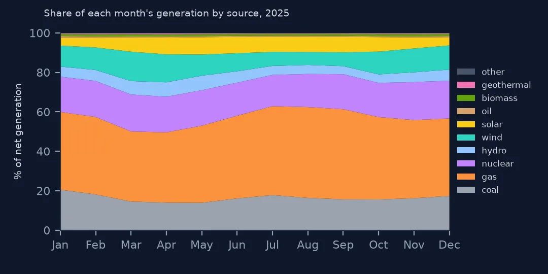
As a share of each month's generation, solar went from 3.9% in January to 8.8% in May, its peak share — in July it produced more energy, but total demand was higher. Wind's share was highest in March (14.9%) and lowest in August (6.6%).

3. Gas fills the gap

tot = mo.sum(axis=1)
print("total generation, TWh:", tot.round(1).to_dict())
print(f"rank correlation of gas with total generation across months: {mo.gas.corr(tot, method='spearman'):+.2f}; "
      f"of nuclear: {mo.nuclear.corr(tot, method='spearman'):+.2f}")

total generation, TWh: {'Jan': 402.0, 'Feb': 338.7, 'Mar': 333.4, 'Apr': 320.8, 'May': 345.6, 'Jun': 395.1, 'Jul': 446.2, 'Aug': 420.7, 'Sep': 368.4, 'Oct': 342.5, 'Nov': 331.6, 'Dec': 380.0}
rank correlation of gas with total generation across months: +0.94; of nuclear: +0.79

Total generation ran from 320.8 TWh in April to 446.2 TWh in July. Gas follows it closely (rank correlation +0.94 across the months): gas plants are the ones that ramp up when demand rises. Nuclear correlates too (+0.79), but because refuelling outages are scheduled in spring and autumn, not because nuclear follows demand.

4. Solar and wind complement each other

print(f"rank correlation of solar with wind across months: {mo.solar.corr(mo.wind, method='spearman'):+.2f}")
both = mo.solar + mo.wind
print(f"wind + solar: lowest {both.min():.1f} TWh in {both.idxmin()}, highest {both.max():.1f} TWh in {both.idxmax()}")

rank correlation of solar with wind across months: -0.72
wind + solar: lowest 54.6 TWh in Sep, highest 73.4 TWh in Mar

Solar and wind move against each other across the year (−0.72): wind is strongest in winter and spring, solar in summer. Together they ranged only from 54.6 TWh in September to 73.4 TWh in March — steadier than either alone.

One state, and nuclear's outages

The data used on this page

The US Energy Information Administration's EIA-923 2025 final monthly generation and fuel data (saved copy).

import io
import zipfile
from pathlib import Path

import geopandas as gpd
import numpy as np
import pandas as pd
import requests

Path("data").mkdir(exist_ok=True)
# EIA-860 (2025, released September 2026), EIA-923 (2025 final) and EIA-860M (August 2026), saved on 15 October 2026.
# Live: https://www.eia.gov/electricity/data/eia860/xls/eia8602025.zip, .../eia923/xls/f923_2025.zip and
# .../eia860m/xls/august_generator2026.xlsx; the annual files move to archive/xls/ when the next year's data appear.
FILES = {"eia860": "eia-860-2025-2026-10-15.zip", "eia923": "eia-923-2025-final-2026-10-15.zip",
         "eia860m": "eia-860m-august-2026-2026-10-15.xlsx"}
for name in FILES.values():
    if not Path(f"data/{name}").exists():
        Path(f"data/{name}").write_bytes(requests.get(f"https://data.spatialworkflow.io/{name}", timeout=600).content)


def read_860(member, sheet=0):
    """One sheet of an EIA-860 workbook; the first row is a title, the last row of some sheets a note."""
    with zipfile.ZipFile(f"data/{FILES['eia860']}") as z:
        d = pd.read_excel(io.BytesIO(z.read(member)), sheet_name=sheet, skiprows=1)
    return d[pd.to_numeric(d["Plant Code"], errors="coerce").notna()]


def read_923(sheet="Page 1 Generation and Fuel Data"):
    with zipfile.ZipFile(f"data/{FILES['eia923']}") as z:
        d = pd.read_excel(io.BytesIO(z.read("EIA923_Schedules_2_3_4_5_M_12_2025_Final.xlsx")), sheet_name=sheet, skiprows=5)
    d.columns = [c.replace("\n", " ") for c in d.columns]
    return d


MER = {"NG": "gas", "COL": "coal", "NUC": "nuclear", "WND": "wind", "SUN": "solar", "HYC": "hydro",
       "DFO": "oil", "RFO": "oil", "PC": "oil", "WOC": "oil", "WWW": "biomass", "MLG": "biomass", "ORW": "biomass",
       "WOO": "biomass", "GEO": "geothermal"}                       # everything else, pumped storage included: "other"
print("EIA-923 file:", FILES["eia923"])

EIA-923 file: eia-923-2025-final-2026-10-15.zip

Example 1: one state's year

tx = g[g["Plant State"] == "TX"]
txm = tx[months].replace(".", np.nan).astype(float).groupby(tx.source).sum().T / 1e6
txm.index = mo.index
print("Texas, TWh:", txm[["gas", "wind", "solar", "coal", "nuclear"]].loc[["Jan", "Apr", "Jul", "Oct"]].round(1).to_dict("index"))

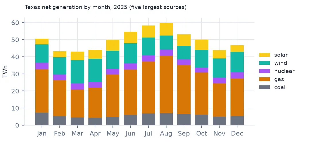
Texas, TWh: {'Jan': {'gas': 25.4, 'wind': 10.8, 'solar': 3.3, 'coal': 7.3, 'nuclear': 3.8}, 'Apr': {'gas': 17.6, 'wind': 13.6, 'solar': 5.2, 'coal': 4.3, 'nuclear': 3.3}, 'Jul': {'gas': 30.3, 'wind': 10.4, 'solar': 7.1, 'coal': 6.8, 'nuclear': 3.7}, 'Oct': {'gas': 24.7, 'wind': 10.4, 'solar': 6.0, 'coal': 6.1, 'nuclear': 2.8}}

In Texas, wind generated 13.6 TWh in April, nearly as much as gas (17.6); in July gas rose to 30.3 TWh while wind stayed near 10. Solar doubled from January (3.3) to July (7.1). Nuclear barely moved; coal dropped in April (4.3) and recovered in summer.

Example 2: nuclear refuelling

nuc = mo.nuclear
print(f"nuclear: lowest {nuc.min():.1f} TWh in {nuc.idxmin()}, highest {nuc.max():.1f} TWh in {nuc.idxmax()}")

nuclear: lowest 57.9 TWh in Apr, highest 72.6 TWh in Dec

Nuclear's lowest month was April (57.9 TWh) and its highest December (72.6): reactors refuel in the mild seasons, when the lost output matters least.

Why the year has this shape

Electricity demand in the US has two peaks — air conditioning in July and August, heating and lighting in December and January — and two troughs in spring and autumn. Plants that cannot follow demand (nuclear, which runs flat out; wind and solar, which follow the weather) produce what they produce, and the dispatchable fleet, mostly gas and some coal, makes up the difference. The monthly table shows that division of labour plainly: gas and coal rise and fall with the total, the others follow their own calendars.

The seasonal complementarity of wind and solar is a property of the US climate, strong in the Plains and Texas, and it is part of why grids with a lot of both need less storage than grids with only one.

Pitfalls in the monthly columns

• The dots. Monthly columns are text because missing months are written as "."; see EIA-923 monthly values are dots.
• Annual reporters. Plants that report once a year have their months estimated by EIA, so their seasonal shape is modelled.
• Net generation. Pumped storage and idle plants are negative; sum them in totals but leave them out of a source chart.
• Days per month. February has fewer days; divide by hours in the month for average power if you compare months.

Internal links

• How to calculate each state's generation mix — the annual totals
• EIA-923 monthly values are dots — why .replace(".", np.nan) is there
• Solar irradiance explained — why solar peaks in summer

FAQ

In which month does the US generate the most electricity?

July: 446.2 TWh of net generation in 2025, against 320.8 TWh in April.

When does wind produce the most electricity in the US?

In spring and winter; in 2025 the peak was March (49.7 TWh) and the low September (26.0 TWh).