
How to Map US Power Plants from EIA-860 Data in Python
On this page
Problem statement
Every power plant in the United States of 1 MW or more files form EIA-860 with the Energy Information Administration each year: where it is, who owns it, and every generator in it, with its technology, fuel and capacity. The 2025 release covers 27,918 operating generators at 14,327 plants, 1,376.7 GW in all, and it is the standard source for a map of the US power fleet. It arrives as Excel workbooks with a title row above the header, a note below the data, numbers stored as text and one row per generator rather than per plant. This guide reads it into GeoPandas, collapses generators to plants and maps them by technology.
Quick answer
Read the plant sheet (locations) and the generator sheet (capacity, technology) with skiprows=1, drop the footer note, convert capacity and coordinates with pd.to_numeric(errors="coerce"), sum generators to plants, and join on Plant Code.
gen["MW"] = pd.to_numeric(gen["Nameplate Capacity (MW)"], errors="coerce")
by_plant = gen.groupby("Plant Code").agg(MW=("MW", "sum"), group=("group", lambda s: s.loc[gen.loc[s.index, "MW"].idxmax()]))
p = plants.merge(by_plant, on="Plant Code", how="inner")
p["Latitude"], p["Longitude"] = pd.to_numeric(p.Latitude, errors="coerce"), pd.to_numeric(p.Longitude, errors="coerce")
pts = gpd.GeoDataFrame(p, geometry=gpd.points_from_xy(p.Longitude, p.Latitude), crs=4326).dropna(subset=["Latitude"])
print(f"{len(pts):,} operating plants, {pts.MW.sum() / 1000:,.0f} GW nameplate")
print(pts.groupby("group").agg(plants=("MW", "size"), GW=("MW", lambda s: round(s.sum() / 1000, 1))).sort_values("GW", ascending=False).to_string())
14,327 operating plants, 1,377 GW nameplate
plants GW
group
gas 1969 563.1
coal 201 195.0
solar 7168 163.2
wind 1358 159.9
nuclear 56 105.1
hydro 1395 80.9
storage 608 55.6
oil 844 32.5
biomass 582 12.3
other 81 5.1
geothermal 65 4.1
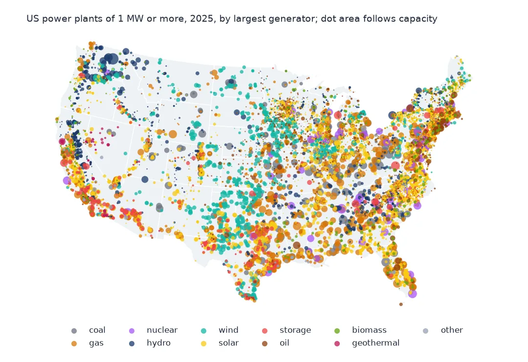
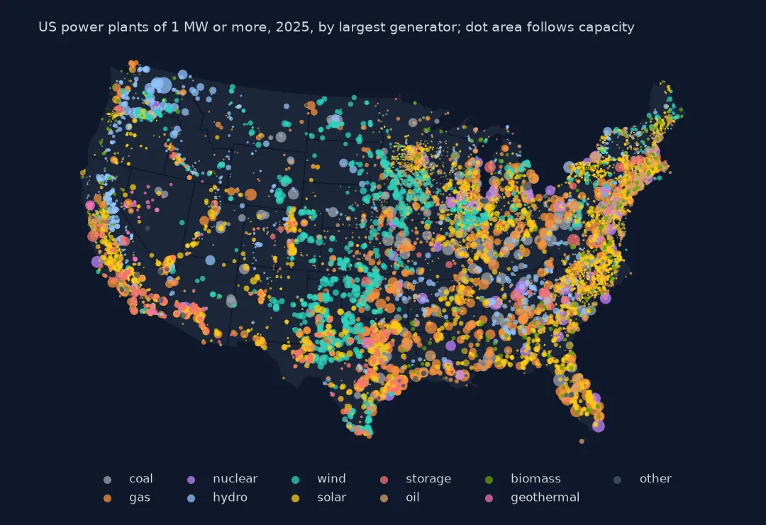
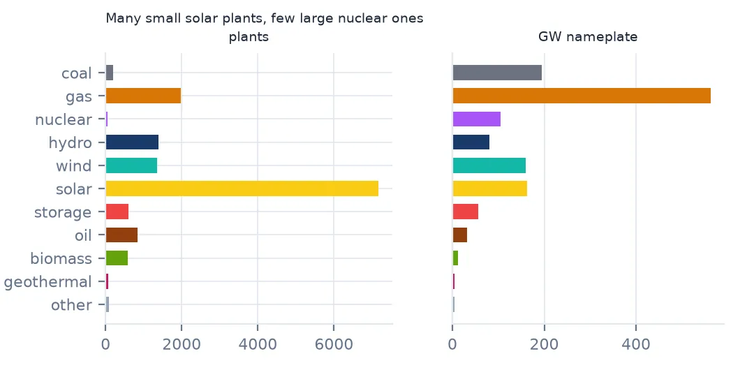
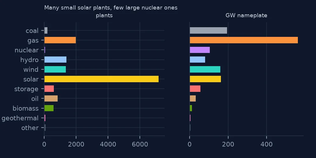
14,327 operating plants hold 1,377 GW of nameplate capacity. Gas has the most capacity (563.1 GW) at 1,969 plants; solar has the most plants (7,168) with less than a third of gas's capacity; 56 nuclear plants hold 105.1 GW. Each plant is labelled by the technology of its largest generator.
From workbook rows to plant points
1. Read the plant and generator sheets
print(f"plant sheet: {len(plants):,} rows, {plants.shape[1]} columns; generator sheet (operable): {len(gen):,} generators")
print("generators per plant:", gen.groupby("Plant Code").size().describe()[["50%", "max"]].to_dict())
plant sheet: 17,349 rows, 42 columns; generator sheet (operable): 27,918 generators
generators per plant: {'50%': 1.0, 'max': 73.0}
The plant sheet has 17,349 rows because it lists every plant with a generator in any status, including proposed and retired ones; the operable generator sheet has 27,918 rows. The median plant has a single generator; the largest has 73.
2. Clean the numbers EIA stores as text
raw = read_860("2___Plant_Y2025.xlsx")
bad = raw[pd.to_numeric(raw.Latitude, errors="coerce").isna()]
print(f"latitudes that are not numbers: {len(bad)}; examples: {bad.Latitude.astype(str).unique()[:3].tolist()}")
with zipfile.ZipFile(f"data/{FILES['eia860']}") as z:
    rawg = pd.read_excel(io.BytesIO(z.read("3_1_Generator_Y2025.xlsx")), sheet_name="Operable", skiprows=1)
print(f"generator rows as read: {len(rawg):,}; the last one: {str(rawg['Utility ID'].iloc[-1])[:58]}...")
latitudes that are not numbers: 28; examples: [' ']
generator rows as read: 27,919; the last one: NOTE: Information on planned capacity changes are data rep...
28 latitudes are a single space — plants without coordinates yet — and would make the whole column text if read as-is. The generator sheet as read has 27,919 rows: the last is a note about planned capacity changes, sitting in the Utility ID column. The setup's read_860 keeps only rows whose plant code is a number, which drops it.
3. One technology per plant
mixed = gen.groupby("Plant Code").group.nunique()
print(f"plants with more than one technology group: {(mixed > 1).sum():,} ({(mixed > 1).mean():.1%}); "
      f"their share of capacity: {gen[gen['Plant Code'].isin(mixed[mixed > 1].index)].MW.sum() / gen.MW.sum():.1%}")
plants with more than one technology group: 906 (6.3%); their share of capacity: 14.2%
906 plants (6.3%) combine technologies — solar with batteries, gas turbines beside a coal unit — and they hold 14.2% of capacity. Labelling each by its largest generator is a simplification; a capacity map by technology should sum generators, not plants.
4. Project and map
l48 = pts[~pts.State.isin(["AK", "HI"])].to_crs(5070)
print(f"lower 48: {len(l48):,} plants; plants in Alaska and Hawaii: {len(pts) - len(l48)}")
print("largest plants:", pts.nlargest(5, "MW")[["Plant Name", "State", "group", "MW"]].round(0).to_dict("records"))
lower 48: 14,101 plants; plants in Alaska and Hawaii: 226
largest plants: [{'Plant Name': 'Grand Coulee', 'State': 'WA', 'group': 'hydro', 'MW': 6809.0}, {'Plant Name': 'Vogtle', 'State': 'GA', 'group': 'nuclear', 'MW': 4658.0}, {'Plant Name': 'West County Energy Center', 'State': 'FL', 'group': 'gas', 'MW': 4263.0}, {'Plant Name': 'Palo Verde', 'State': 'AZ', 'group': 'nuclear', 'MW': 4210.0}, {'Plant Name': 'W A Parish', 'State': 'TX', 'group': 'coal', 'MW': 4008.0}]
226 plants are in Alaska and Hawaii, mapped separately or left out of a lower-48 map. The largest plant is Grand Coulee Dam in Washington (6,809 MW), followed by the Vogtle nuclear plant in Georgia (4,658 MW).
States and plant sizes
The data used on this page
The US Energy Information Administration's EIA-860 annual electric generator report for 2025 (plants of 1 MW or more), released in September 2026 — saved copies of the files, read from this site — and Census Bureau 2023 cartographic boundary states for the map.
import io
import zipfile
from pathlib import Path

import geopandas as gpd
import numpy as np
import pandas as pd
import requests

Path("data").mkdir(exist_ok=True)
# EIA-860 (2025, released September 2026), EIA-923 (2025 final) and EIA-860M (August 2026), saved on 15 October 2026.
# Live: https://www.eia.gov/electricity/data/eia860/xls/eia8602025.zip, .../eia923/xls/f923_2025.zip and
# .../eia860m/xls/august_generator2026.xlsx; the annual files move to archive/xls/ when the next year's data appear.
FILES = {"eia860": "eia-860-2025-2026-10-15.zip", "eia923": "eia-923-2025-final-2026-10-15.zip",
         "eia860m": "eia-860m-august-2026-2026-10-15.xlsx"}
for name in FILES.values():
    if not Path(f"data/{name}").exists():
        Path(f"data/{name}").write_bytes(requests.get(f"https://data.spatialworkflow.io/{name}", timeout=600).content)


def read_860(member, sheet=0):
    """One sheet of an EIA-860 workbook; the first row is a title, the last row of some sheets a note."""
    with zipfile.ZipFile(f"data/{FILES['eia860']}") as z:
        d = pd.read_excel(io.BytesIO(z.read(member)), sheet_name=sheet, skiprows=1)
    return d[pd.to_numeric(d["Plant Code"], errors="coerce").notna()]


def read_923(sheet="Page 1 Generation and Fuel Data"):
    with zipfile.ZipFile(f"data/{FILES['eia923']}") as z:
        d = pd.read_excel(io.BytesIO(z.read("EIA923_Schedules_2_3_4_5_M_12_2025_Final.xlsx")), sheet_name=sheet, skiprows=5)
    d.columns = [c.replace("\n", " ") for c in d.columns]
    return d


GROUP = {"Conventional Steam Coal": "coal", "Coal Integrated Gasification Combined Cycle": "coal",
         "Natural Gas Fired Combined Cycle": "gas", "Natural Gas Fired Combustion Turbine": "gas",
         "Natural Gas Steam Turbine": "gas", "Natural Gas Internal Combustion Engine": "gas",
         "Natural Gas with Compressed Air Storage": "gas", "Other Natural Gas": "gas", "Nuclear": "nuclear",
         "Onshore Wind Turbine": "wind", "Offshore Wind Turbine": "wind", "Solar Photovoltaic": "solar",
         "Solar Thermal with or without Energy Storage": "solar", "Conventional Hydroelectric": "hydro",
         "Batteries": "storage", "Hydroelectric Pumped Storage": "storage", "Flywheels": "storage",
         "Petroleum Liquids": "oil", "Petroleum Coke": "oil", "Wood/Wood Waste Biomass": "biomass",
         "Landfill Gas": "biomass", "Municipal Solid Waste": "biomass", "Other Waste Biomass": "biomass",
         "Geothermal": "geothermal"}
gen = read_860("3_1_Generator_Y2025.xlsx", "Operable")
gen["MW"] = pd.to_numeric(gen["Nameplate Capacity (MW)"], errors="coerce")
gen["group"] = gen.Technology.map(GROUP).fillna("other")
plants = read_860("2___Plant_Y2025.xlsx")
f = Path("data/cb_2023_us_state_20m.zip")
if not f.exists():
    f.write_bytes(requests.get("https://www2.census.gov/geo/tiger/GENZ2023/shp/cb_2023_us_state_20m.zip", timeout=300).content)
states = gpd.read_file(f)
states = states[~states.STUSPS.isin(["PR"])]
print(f"{len(plants):,} plants, {len(gen):,} operable generators, {gen.MW.sum() / 1000:,.1f} GW nameplate")
17,349 plants, 27,918 operable generators, 1,376.7 GW nameplate
Example 1: capacity by state
st = gen.groupby(["State", "group"]).MW.sum().unstack(fill_value=0) / 1000
st["total"] = st.sum(axis=1)
print(st.sort_values("total", ascending=False).head(5).round(1).to_string())
group biomass coal gas geothermal hydro nuclear oil other solar storage wind total
State
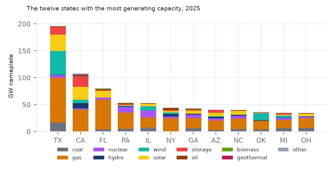
TX 0.4 16.6 83.0 0.0 0.7 5.1 0.9 0.5 30.8 14.1 43.9 196.0
CA 1.1 0.1 40.2 2.9 10.0 2.3 0.6 1.2 23.9 18.6 6.5 107.4
FL 1.1 3.7 55.3 0.0 0.0 3.9 2.0 0.3 12.3 1.2 0.0 79.9
PA 0.5 5.2 29.9 0.0 0.9 10.5 1.7 0.1 1.1 1.5 1.6 53.1
IL 0.1 7.4 18.8 0.0 0.0 12.4 0.8 0.1 4.4 0.1 8.5 52.5
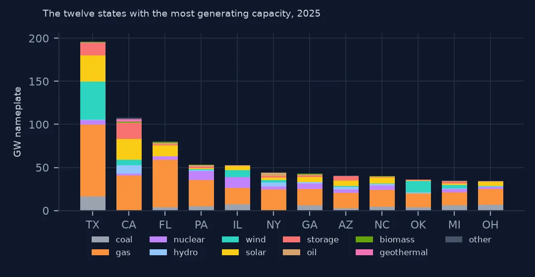
Texas has 196.0 GW, almost twice California's 107.4 GW: 83.0 GW of gas, 43.9 of wind, 30.8 of solar and 14.1 of batteries. California has the most battery capacity (18.6 GW) and Illinois the most nuclear in this list (12.4 GW).
Example 2: how big plants are
sz = pts.groupby("group").MW.median().sort_values(ascending=False)
print("median plant nameplate, MW:", sz.round(1).to_dict())
print(f"plants under 5 MW: {(pts.MW < 5).mean():.1%} of plants, {pts[pts.MW < 5].MW.sum() / pts.MW.sum():.1%} of capacity")
median plant nameplate, MW: {'nuclear': 1849.2, 'coal': 763.2, 'wind': 100.0, 'gas': 71.2, 'geothermal': 35.0, 'other': 31.9, 'storage': 10.4, 'hydro': 7.5, 'oil': 6.6, 'biomass': 6.4, 'solar': 3.4}
plants under 5 MW: 42.6% of plants, 1.0% of capacity
The median nuclear plant is 1,849.2 MW and the median solar plant 3.4 MW. 42.6% of plants are under 5 MW, but together they hold only 1.0% of capacity — on a map they are most of the dots and almost none of the power, so size the points by capacity.
What EIA-860 covers
EIA-860 is a census of generators of 1 MW or more connected to the grid, filed by the plant's operator. It records the physical fleet: location, technology, prime mover, fuel, capacity, operating and planned retirement dates. It does not record what plants generate — that is EIA-923 — and it leaves out generation below 1 MW, which is where nearly all rooftop solar sits. A map from EIA-860 is a map of utility-scale power.
The file is organised around generators because that is the unit that is built, repowered and retired; a plant is a site with one or more of them. Most analysis needs both levels: generators for capacity by technology, plants for location.
Pitfalls in the workbook
- Title and note rows.
skiprows=1for the header, and drop the trailing note, or one stray text row turns numeric columns into objects. - Blank strings. EIA writes a space for missing values;
pd.to_numeric(errors="coerce")turns them into NaN. - Plant codes are numbers in one file and strings in another. Cast both sides of a join to
int. - Status. The operable sheet includes generators on standby or out of service; filter
Statusif you want only those in use.
Internal links
- EIA-860 and EIA-923 explained — what the forms record
- Nameplate or summer capacity — which capacity to sum
- How to measure distance to the grid for renewable siting — plants and lines in siting work
FAQ
How many power plants are there in the US?
EIA-860 for 2025 lists 14,327 plants with operable generators of 1 MW or more, holding 1,376.7 GW of nameplate capacity.
Does EIA-860 include rooftop solar?
No. It covers generators of 1 MW or more; small-scale solar is estimated separately by EIA.