
How to Calculate Capacity Factors of Real Power Plants from EIA Data
On this page
Problem statement
A capacity factor — what a plant generated divided by what it could have generated running flat out all year — is the single number that separates a nuclear plant from a peaking gas turbine, and a good wind site from a poor one. Computing it for real plants needs capacity from EIA-860 and generation from EIA-923, and the two files are organised differently: capacity is per generator, generation per plant and fuel, and plants add and lose generators during the year. This guide computes 2025 capacity factors for the 12,095 plants where the join is clean, by technology, and shows the choices that change the numbers.
Quick answer
Keep plants whose generators are all one technology and all in service for the whole year, sum their nameplate capacity, join annual net generation by plant code, and divide by capacity times the hours in the year. Report the fleet figure as total generation over total capacity, not the mean of plant figures.
g = read_923()
full = gen[(pd.to_numeric(gen["Operating Year"], errors="coerce") < 2025)]          # in service all of 2025
single = full.groupby("Plant Code").group.nunique().pipe(lambda s: s[s == 1].index)
cap = full[full["Plant Code"].isin(single)].groupby("Plant Code").agg(MW=("MW", "sum"), group=("group", "first"))
late = gen[pd.to_numeric(gen["Operating Year"], errors="coerce") >= 2025]["Plant Code"].unique()
cap = cap[~cap.index.isin(late)]                                                      # no part-year units
gen_mwh = g.groupby("Plant Id")["Net Generation (Megawatthours)"].sum()
cf = cap.join(gen_mwh.rename("MWh"), how="inner")
cf["cf"] = cf.MWh / (cf.MW * 8760)
fleet = cf.groupby("group").apply(lambda d: d.MWh.sum() / (d.MW.sum() * 8760), include_groups=False)
print(f"{len(cf):,} single-technology plants in service all year")
print("fleet capacity factor, 2025:", fleet.sort_values(ascending=False).round(3).to_dict())
12,095 single-technology plants in service all year
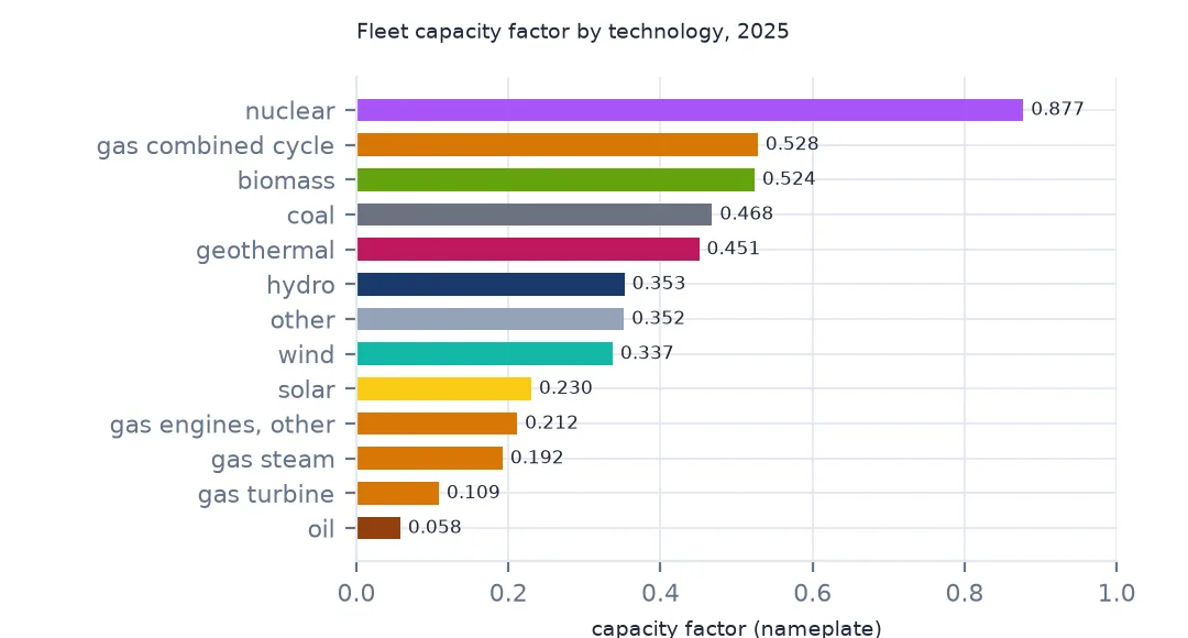
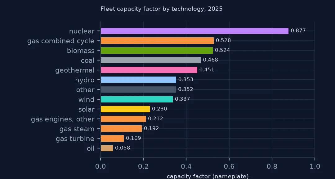
fleet capacity factor, 2025: {'nuclear': 0.877, 'gas combined cycle': 0.528, 'biomass': 0.524, 'coal': 0.468, 'geothermal': 0.451, 'hydro': 0.353, 'other': 0.352, 'wind': 0.337, 'solar': 0.23, 'gas': 0.212, 'gas steam': 0.192, 'gas turbine': 0.109, 'oil': 0.058, 'storage': -0.019}
For 2025 the fleet capacity factors are: nuclear 0.877, gas combined cycle 0.528, biomass 0.524, coal 0.468, geothermal 0.451, hydro 0.353, wind 0.337, solar 0.23, gas steam units 0.192, gas turbines 0.109 and oil 0.058. Storage comes out negative (−0.019), because batteries consume more than they return.
Joining capacity to generation
1. Capacity from EIA-860, generation from EIA-923
print(f"plants with capacity: {len(cap):,}; with generation: {gen_mwh.size:,}; matched: {len(cf):,}")plants with capacity: 12,459; with generation: 14,045; matched: 12,095
12,459 plants pass the capacity filters and 14,045 have generation; 12,095 have both. The plants lost are mostly ones with mixed technologies, which cannot be given a single capacity factor from plant-level generation.
2. Keep plants in service all year
print(f"generators that started in 2025: {len(gen) - len(full):,}, {gen.MW.sum() - full.MW.sum():,.0f} MW")
print(f"plants left out for a part-year unit: {len(late):,}")
generators that started in 2025: 1,090, 57,729 MW
plants left out for a part-year unit: 920
1,090 generators, 57,729 MW, started during 2025. A plant that added a unit in, say, October has a year's capacity in the denominator and three months of that unit's output in the numerator, so 920 plants with any part-year unit are left out rather than prorated.
3. Plant against fleet
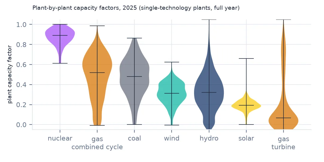
d = cf.groupby("group").cf.describe(percentiles=[0.1, 0.5, 0.9])[["count", "10%", "50%", "90%"]]
print(d.round(3).to_string())
count 10% 50% 90%
group
biomass 525.0 0.028 0.530 0.810
coal 148.0 0.224 0.480 0.701
gas 415.0 0.003 0.042 0.901
gas combined cycle 417.0 0.146 0.519 0.731
gas steam 126.0 0.003 0.212 0.593
gas turbine 581.0 0.002 0.067 0.735
geothermal 51.0 0.282 0.469 0.747
hydro 1324.0 0.077 0.323 0.562
nuclear 49.0 0.770 0.890 0.960
oil 705.0 0.000 0.002 0.098
other 69.0 0.103 0.407 0.772
solar 6043.0 0.128 0.192 0.258
storage 376.0 -0.025 -0.010 -0.002
wind 1266.0 0.166 0.312 0.443
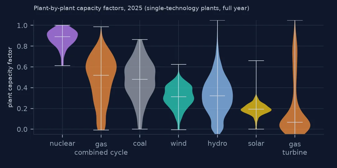
The spread inside a technology is as informative as the average. Nuclear plants sit between 0.77 and 0.96 (10th and 90th percentiles). Solar is tight, 0.128 to 0.258, because sunshine varies less than wind, whose plants range from 0.166 to 0.443. Gas turbines have a median of 0.067: they are built to run a few hundred hours a year at peak demand, so a low figure is their job, not a failure.
4. Impossible values
print(f"capacity factor above 1: {(cf.cf > 1).sum()} plants; below 0: {(cf.cf < 0).sum()}")
print(cf[cf.cf > 1].nlargest(3, "cf")[["group", "MW", "MWh", "cf"]].round(2).to_string())
capacity factor above 1: 10 plants; below 0: 432
group MW MWh cf
Plant Code
65028.0 storage 51.8 1034197.0 2.28
594.0 oil 18.6 255871.0 1.57
58696.0 hydro 1.5 20168.0 1.53
10 plants exceed 1, which is impossible, and 432 are below 0. The largest overshoot is a storage plant reporting more output than its capacity allows; for the others, reported generation and listed capacity do not fit together, a reporting problem to check plant by plant. Check outliers before averaging, and prefer fleet totals, which they barely move.
The denominator and the sun
The data used on this page
The US Energy Information Administration's EIA-860 generator inventory and EIA-923 net generation for 2025 (saved copies).
import io
import zipfile
from pathlib import Path

import geopandas as gpd
import numpy as np
import pandas as pd
import requests

Path("data").mkdir(exist_ok=True)
# EIA-860 (2025, released September 2026), EIA-923 (2025 final) and EIA-860M (August 2026), saved on 15 October 2026.
# Live: https://www.eia.gov/electricity/data/eia860/xls/eia8602025.zip, .../eia923/xls/f923_2025.zip and
# .../eia860m/xls/august_generator2026.xlsx; the annual files move to archive/xls/ when the next year's data appear.
FILES = {"eia860": "eia-860-2025-2026-10-15.zip", "eia923": "eia-923-2025-final-2026-10-15.zip",
         "eia860m": "eia-860m-august-2026-2026-10-15.xlsx"}
for name in FILES.values():
    if not Path(f"data/{name}").exists():
        Path(f"data/{name}").write_bytes(requests.get(f"https://data.spatialworkflow.io/{name}", timeout=600).content)


def read_860(member, sheet=0):
    """One sheet of an EIA-860 workbook; the first row is a title, the last row of some sheets a note."""
    with zipfile.ZipFile(f"data/{FILES['eia860']}") as z:
        d = pd.read_excel(io.BytesIO(z.read(member)), sheet_name=sheet, skiprows=1)
    return d[pd.to_numeric(d["Plant Code"], errors="coerce").notna()]


def read_923(sheet="Page 1 Generation and Fuel Data"):
    with zipfile.ZipFile(f"data/{FILES['eia923']}") as z:
        d = pd.read_excel(io.BytesIO(z.read("EIA923_Schedules_2_3_4_5_M_12_2025_Final.xlsx")), sheet_name=sheet, skiprows=5)
    d.columns = [c.replace("\n", " ") for c in d.columns]
    return d


GROUP = {"Conventional Steam Coal": "coal", "Coal Integrated Gasification Combined Cycle": "coal",
         "Natural Gas Fired Combined Cycle": "gas", "Natural Gas Fired Combustion Turbine": "gas",
         "Natural Gas Steam Turbine": "gas", "Natural Gas Internal Combustion Engine": "gas",
         "Natural Gas with Compressed Air Storage": "gas", "Other Natural Gas": "gas", "Nuclear": "nuclear",
         "Onshore Wind Turbine": "wind", "Offshore Wind Turbine": "wind", "Solar Photovoltaic": "solar",
         "Solar Thermal with or without Energy Storage": "solar", "Conventional Hydroelectric": "hydro",
         "Batteries": "storage", "Hydroelectric Pumped Storage": "storage", "Flywheels": "storage",
         "Petroleum Liquids": "oil", "Petroleum Coke": "oil", "Wood/Wood Waste Biomass": "biomass",
         "Landfill Gas": "biomass", "Municipal Solid Waste": "biomass", "Other Waste Biomass": "biomass",
         "Geothermal": "geothermal"}
gen = read_860("3_1_Generator_Y2025.xlsx", "Operable")
gen["MW"] = pd.to_numeric(gen["Nameplate Capacity (MW)"], errors="coerce")
gen["group"] = gen.Technology.map(GROUP).fillna("other")
plants = read_860("2___Plant_Y2025.xlsx")
gen["group"] = gen.Technology.map({"Natural Gas Fired Combined Cycle": "gas combined cycle",
                                    "Natural Gas Fired Combustion Turbine": "gas turbine",
                                    "Natural Gas Steam Turbine": "gas steam"}).fillna(gen.group)   # gas split by kind
print(f"{len(plants):,} plants, {len(gen):,} operable generators, {gen.MW.sum() / 1000:,.1f} GW nameplate")
17,349 plants, 27,918 operable generators, 1,376.7 GW nameplate
Example 1: summer capacity instead of nameplate
full_s = full.assign(S=pd.to_numeric(full["Summer Capacity (MW)"], errors="coerce"))
cap_s = full_s[full_s["Plant Code"].isin(cf.index)].groupby("Plant Code").S.sum()
cf2 = cf.join(cap_s)
alt = cf2.groupby("group").apply(lambda d: d.MWh.sum() / (d.S.sum() * 8760), include_groups=False)
print("fleet capacity factor on summer capacity:", alt.sort_values(ascending=False).round(3).to_dict())
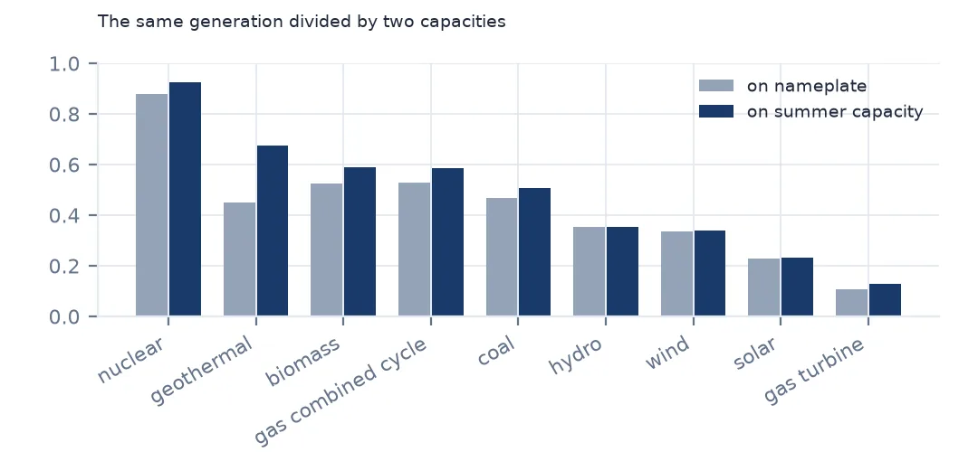
fleet capacity factor on summer capacity: {'nuclear': 0.924, 'geothermal': 0.675, 'biomass': 0.59, 'gas combined cycle': 0.587, 'coal': 0.506, 'other': 0.382, 'hydro': 0.355, 'wind': 0.338, 'solar': 0.231, 'gas': 0.219, 'gas steam': 0.208, 'gas turbine': 0.129, 'oil': 0.068, 'storage': -0.019}
On summer capacity — the output a unit can sustain in summer heat — nuclear rises to 0.924 and geothermal to 0.675, because their summer ratings sit below nameplate; wind and solar barely change. Which capacity is in the denominator should be stated with every figure (nameplate or summer capacity).
Example 2: solar by latitude
sol = cf[cf.group == "solar"].join(plants.set_index("Plant Code").Latitude.pipe(pd.to_numeric, errors="coerce"))
sol["band"] = pd.cut(sol.Latitude, [20, 30, 35, 40, 45, 50], labels=["20-30N", "30-35N", "35-40N", "40-45N", "45-50N"])
print("median solar capacity factor by latitude band:", sol.groupby("band", observed=True).cf.median().round(3).to_dict())
median solar capacity factor by latitude band: {'20-30N': 0.22, '30-35N': 0.218, '35-40N': 0.199, '40-45N': 0.178, '45-50N': 0.191}
Solar plants south of 30°N had a median capacity factor of 0.22 in 2025, against 0.178 between 40° and 45°N. The 45–50°N band (0.191) is higher than the band south of it, a reminder that cloud and tracking matter as well as latitude.
What a capacity factor measures
A capacity factor mixes two things: how much of the time a plant could run, and how much of that time it was asked to. For wind and solar the first dominates — the resource sets the output, and the concept guide explains why. For dispatchable plants the second does: a combined-cycle gas plant at 0.528 could run far more, but runs when it is the cheapest option, and coal's 0.468 reflects being displaced by gas and renewables as much as anything about the plants themselves.
That is why capacity factors compare well within a technology and badly across them. A wind plant at 0.44 is excellent; a nuclear plant at 0.44 has had a long outage.
Choices that change the number
- Nameplate, summer or AC/DC. Solar nameplate in EIA-860 is AC; a DC-based figure is lower.
- Hours in the year. A leap year has 24 more; use the year's real length.
- Retirements and repowering. A plant that retired a unit mid-year has the same problem as one that added one; check
Retirement Yeartoo if you use the retired sheet. - Net, not gross. EIA-923 is net of the plant's own use, so thermal plants come out slightly lower than gross figures in other sources.
Internal links
- Capacity factor explained — the concept
- Nameplate or summer capacity — the denominator matters
- How to model PV output with pvlib — a modelled capacity factor for one site
FAQ
What is the capacity factor of US nuclear plants?
0.877 on nameplate capacity in 2025 across 49 plants that ran all year, or 0.924 on summer capacity.
What is a typical solar capacity factor in the US?
The 2025 fleet figure is 0.23 on AC nameplate, with the 10th to 90th percentile of plants between 0.128 and 0.258.