
How to find which species occur in protected areas
On this page
Problem statement
"How many species does this park protect?" is a spatial join with three traps in it. Records inside a park boundary are not the same as species the park protects; the count depends entirely on how much recording has happened inside versus outside; and a record with a 10 km uncertainty radius cannot be assigned to a 5 km² reserve at all.
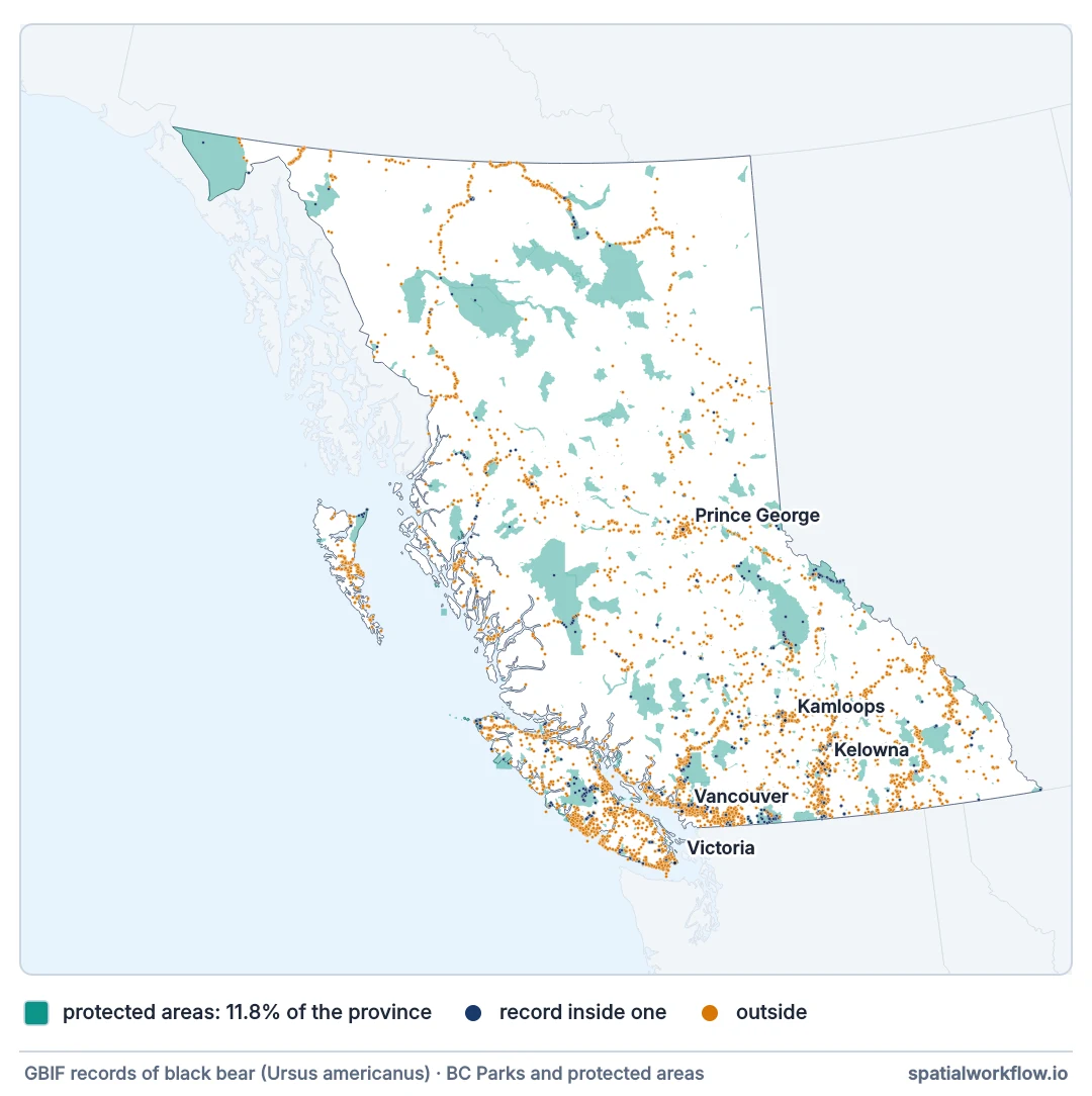
This guide joins British Columbia's mammal records to its 929 protected areas, and measures how much of the answer is recording effort.
Quick answer
Join, count, and immediately compare with effort:
import numpy as np, pandas as pd, geopandas as gpd
from gbif import search
from pa import protected_areas
from shapely.validation import make_valid

pas = protected_areas()                                   # BC Albers, EPSG:3005
pas["geometry"] = [make_valid(g) for g in pas.geometry]
pas["km2"] = pas.area / 1e6

bears = search(taxonKey=2433407, country="CA", stateProvince="British Columbia",
               hasCoordinate="true")
pts = gpd.GeoDataFrame(bears, crs=4326,
                       geometry=gpd.points_from_xy(bears.decimalLongitude,
                                                   bears.decimalLatitude)).to_crs(3005)

hit = gpd.sjoin(pts, pas[["PROTECTED_LANDS_NAME", "km2", "geometry"]],
                predicate="within", how="left")
inside = hit.PROTECTED_LANDS_NAME.notna()

print(f"{len(pts):,} records; {inside.sum():,} inside a protected area "
      f"({inside.mean():.1%})")
print(f"protected land is {pas.union_all().area / 1e6 / 944_735:.1%} of the province")
print(f"records are over-represented in protected areas by "
      f"{inside.mean() / (pas.union_all().area / 1e6 / 944_735):.1f}×")
7,560 records; 1,069 inside a protected area (14.1%)
protected land is 11.8% of the province
records are over-represented in protected areas by 1.2×
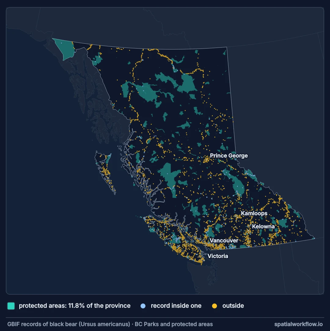
Fourteen per cent of the records fall inside protected areas, which hold 11.8% of the province: an over-representation of 1.2×, much milder than expected. It is worth measuring rather than assuming — for the same records, being within ten kilometres of a town is an eleven-fold over-representation. Parks attract recording, but in this province roads attract it far more.
Repair polygons, use within, filter by uncertainty
1. Repair the polygons first
Invalid geometry makes sjoin unreliable and union_all fail. Forty of these 929 polygons are invalid as published.
2. Use within, not intersects, for points
They are the same for points except on a boundary, and being explicit documents the intent.
3. Drop records whose uncertainty exceeds the site
A record with a 10 km radius cannot be attributed to a 2 km² reserve. That filter removes most records from small sites, which is the honest outcome.
4. Count species, not records
A site's value is the species list. Records per site is a measure of visitor numbers.
5. Compare against effort, not against area
Species per site rises with records per site. Rarefy, or compare sites at a common sample size.
6. Say what "protects" means
A species recorded inside a boundary may be a vagrant, may depend on habitat outside it, and may be declining inside it. The join supports "recorded in", and nothing stronger.
Per-site species lists and effort
The data used on this page
Records come from the GBIF API via gbif.search, the paging function from the download guide plus eventDate and countryCode. Climate is WorldClim 2.1 bioclim at 10′ in bio/wc/; pa.protected_areas() is British Columbia's protected-area layer (EPSG:3005). GBIF changes daily, so the setup answers each request with the reply it got on 9 October 2026.
import hashlib
import io
import os
import zipfile

import requests

# GBIF adds and revises records daily. So that the numbers below reproduce, every GBIF request on
# this page is answered from the reply it got on 9 October 2026 (one file per request, named by a
# SHA-1 of its URL); any other request, or all of them once these lines are deleted, goes live.
SAVED = zipfile.ZipFile(io.BytesIO(requests.get(
    "https://data.spatialworkflow.io/gbif-api-2026-10-09.zip", timeout=300).content))
live_get = requests.get


def saved_get(url, params=None, **kwargs):
    prepared = requests.Request("GET", url, params=params).prepare()
    try:
        body = SAVED.read(hashlib.sha1(prepared.url.encode()).hexdigest()[:16] + ".json")
    except KeyError:
        return live_get(url, params=params, **kwargs)
    reply = requests.models.Response()
    reply.status_code, reply._content, reply.url = 200, body, prepared.url
    reply.headers["Content-Type"] = "application/json"
    return reply


requests.get = saved_get

os.makedirs("bio/wc", exist_ok=True)
with open("gbif.py", "w") as f:
    f.write('''
import pandas as pd, requests

API = "https://api.gbif.org/v1"
MAX_OFFSET = 100_000
FIELDS = ["key", "species", "speciesKey", "decimalLongitude", "decimalLatitude",
          "coordinateUncertaintyInMeters", "year", "month", "basisOfRecord",
          "datasetKey", "institutionCode", "issues", "eventDate", "countryCode"]


def count(**params):
    return requests.get(f"{API}/occurrence/search", params={**params, "limit": 0}, timeout=120).json()["count"]


def search(limit=None, page=300, **params):
    total = count(**params)
    if limit is None and total > MAX_OFFSET:
        raise ValueError(f"{total:,} records exceeds the {MAX_OFFSET:,} offset limit")
    rows, offset = [], 0
    target = total if limit is None else min(limit, total)
    while offset < target:
        body = requests.get(f"{API}/occurrence/search",
                            params={**params, "limit": min(page, target - offset), "offset": offset},
                            timeout=180).json()
        rows += body["results"]
        offset += len(body["results"])
        if body["endOfRecords"] or not body["results"]:
            break
    return pd.DataFrame([{f: r.get(f) for f in FIELDS} for r in rows])
''')
with open("pa.py", "w") as f:
    f.write('''
import os
import geopandas as gpd

URL = ("https://services6.arcgis.com/ubm4tcTYICKBpist/arcgis/rest/services/"
       "British_Columbia_Parks_Ecological_Reserves_and_Protected_Areas/FeatureServer/0/query"
       "?where=1%3D1&outFields=PROTECTED_LANDS_NAME&outSR=3005&f=geojson")


def protected_areas():
    if not os.path.exists("bio/bc_protected.gpkg"):
        gpd.read_file(URL).to_file("bio/bc_protected.gpkg")
    return gpd.read_file("bio/bc_protected.gpkg")
''')
if not os.path.exists("bio/wc/wc2.1_10m_bio_1.tif"):
    blob = requests.get("https://geodata.ucdavis.edu/climate/worldclim/2_1/base/wc2.1_10m_bio.zip", timeout=600).content
    zipfile.ZipFile(io.BytesIO(blob)).extractall("bio/wc")
print(len([n for n in os.listdir("bio/wc") if n.endswith(".tif")]), "WorldClim layers")
19 WorldClim layers
Example 1 — per-site species lists for a whole taxon
TAXA = {2433407: "black bear", 5219153: "coyote", 2440940: "moose",
        2437364: "marmots", 5219173: "grey wolf", 5218864: "American marten"}
mammals = pd.concat([search(taxonKey=k, country="CA", stateProvince="British Columbia",
                            hasCoordinate="true") for k in TAXA],
                    ignore_index=True)
mam = gpd.GeoDataFrame(mammals, crs=4326,
                       geometry=gpd.points_from_xy(mammals.decimalLongitude,
                                                   mammals.decimalLatitude)).to_crs(3005)

joined = gpd.sjoin(mam, pas[["PROTECTED_LANDS_NAME", "km2", "geometry"]],
                   predicate="within", how="inner")
per_site = (joined.groupby("PROTECTED_LANDS_NAME")
            .agg(records=("species", "size"), species=("species", "nunique"),
                 km2=("km2", "first"))
            .sort_values("records", ascending=False))

print(f"{len(mam):,} records of {mam.species.nunique()} species "
      f"across {len(TAXA)} queried taxa")
print(f"{len(joined):,} fall inside {len(per_site)} protected areas")
print(per_site.head(6).round(1).to_string())
17,235 records of 9 species across 6 queried taxa
2,689 fall inside 295 protected areas
records species km2
PROTECTED_LANDS_NAME
GARIBALDI PARK 198 3 1886.6
E.C. MANNING PARK 161 6 837.9
KALAMALKA LAKE PARK 131 3 32.2
BOWRON LAKE PARK 116 5 1397.7
WELLS GRAY PARK 86 5 5404.1
SOUTH OKANAGAN GRASSLANDS PROTECTED AREA 79 4 93.3
Example 2 — the uncertainty filter
small = pas[pas.km2 < 10]
print(f"{len(small)} sites under 10 km²; median {small.km2.median():.2f} km²")

radius = mam.coordinateUncertaintyInMeters
for limit_km, label in [(None, "no filter"), (10, "uncertainty <= 10 km"),
                        (1, "uncertainty <= 1 km"), (0.1, "uncertainty <= 100 m")]:
    if limit_km is None:
        sel = mam
    else:
        sel = mam[radius.fillna(np.inf) <= limit_km * 1000]
    j = gpd.sjoin(sel, small[["PROTECTED_LANDS_NAME", "geometry"]],
                  predicate="within", how="inner")
    print(f"  {label:<24} {len(sel):>7,} records usable, "
          f"{len(j):>5,} in small sites, "
          f"{j.PROTECTED_LANDS_NAME.nunique():>3} sites with any")
637 sites under 10 km²; median 1.04 km²
no filter 17,235 records usable, 635 in small sites, 152 sites with any
uncertainty <= 10 km 13,570 records usable, 502 in small sites, 136 sites with any
uncertainty <= 1 km 11,988 records usable, 474 in small sites, 126 sites with any
uncertainty <= 100 m 9,007 records usable, 348 in small sites, 104 sites with any
Tightening the filter to a hundred metres roughly halves the usable records and takes nearly half of the small sites' records with them — 635 down to 348, across 104 sites instead of 152. Those are the records that can actually be attributed to a one-square-kilometre reserve. Publishing a species list for such a site without the filter publishes whatever was recorded in the valley around it.
Example 3 — effort, and what survives it
from scipy.special import gammaln

def rarefy(counts, m):
    n = counts.sum()
    if m > n:
        return np.nan
    log_missing = (gammaln(n - counts + 1) - gammaln(n - counts - m + 1)
                   - gammaln(n + 1) + gammaln(n - m + 1))
    return float(len(counts) - np.exp(log_missing).sum())

rows = []
for name, sub in joined.groupby("PROTECTED_LANDS_NAME"):
    counts = sub.species.value_counts().to_numpy().astype(float)
    rows.append({"site": name, "km2": sub.km2.iloc[0], "records": int(counts.sum()),
                 "species": len(counts), "rarefied_50": rarefy(counts, 50)})
sites = pd.DataFrame(rows)

usable = sites[sites.rarefied_50.notna()]
print(f"{len(sites)} sites with records; {len(usable)} with at least 50")
print(f"observed species:  median {usable.species.median():.1f}, "
      f"max {usable.species.max()}")
print(f"rarefied to 50:    median {usable.rarefied_50.median():.2f}, "
      f"max {usable.rarefied_50.max():.2f}")
corr_raw = np.corrcoef(np.log10(usable.records), usable.species)[0, 1]
corr_adj = np.corrcoef(np.log10(usable.records), usable.rarefied_50)[0, 1]
print(f"correlation with log(records): observed {corr_raw:.2f}, "
      f"rarefied {corr_adj:.2f}")
295 sites with records; 13 with at least 50
observed species: median 4.0, max 6
rarefied to 50: median 3.87, max 5.35
correlation with log(records): observed 0.16, rarefied 0.07
Only 13 of the 295 sites with records have the 50 needed to rarefy, which is the real finding: for six mammal taxa across a province of 929 protected areas, almost no site has enough records to compare with another. The effort correlation is weak here (0.16) precisely because the counts are so small — with nine species in the pool and a median of four per site, there is little room for effort to matter.
Recorded in is the only supported claim
Why "recorded in" is the only supported claim
A spatial join tells you a record's coordinate fell inside a polygon. It does not tell you the species breeds there, depends on the site, or would disappear without it — and for wide-ranging species like a bear, a park boundary is a line the animal crosses daily. Gap analysis and representation targets are built on exactly this join, which is why they are always stated as coverage of records or of modelled range, not of populations.
Why protected areas attract records
Parks have access, parking, trails, interpretation and visitors who photograph wildlife. That produces a recording density far above the surrounding landscape and makes any uncorrected comparison between protected and unprotected land meaningless. The over-representation measured above is the size of the problem for this taxon in this province.
Why small sites are the hardest case
The smaller the site, the larger the fraction of candidate records whose uncertainty exceeds it, and the fewer records remain. A 2 km² ecological reserve may end up with a handful of attributable records, which is a true statement about the data and a poor basis for a species list. Aggregating small sites into a class, rather than reporting each, is usually the honest presentation.
Marine sites, overlaps and buffer zones
- Marine sites need marine records; joining terrestrial species to them produces nonsense.
- Overlapping designations mean a record can be "in" several sites; decide whether to count it once.
- Buffer zones and transition areas are separate polygons in some datasets and part of the site in others.
- Site boundaries change: a record from 1990 in a park designated in 2005 was not in a park when it was made.
- Modelled ranges rather than points are the standard input for representation analyses at national scale.
sjoinwith polygons needspredicate="intersects"and an area-weighted interpretation.
Internal links
- Protected area data explained — the polygons and their traps
- Species occurrence data explained — the records
- Sampling bias in occurrence data explained — why parks are over-recorded
- How to correct richness for sampling effort — the correction used here
- Coordinate uncertainty explained — the filter small sites need
- How to count buildings and people exposed to a hazard zone — the same join in hazard work
- Avoided deforestation explained — why inside-versus-outside overstates protection
FAQ
How do I find species recorded in a protected area?
Spatially join cleaned occurrence points to the site polygons and count distinct species per site.
Does a record inside a park mean the park protects the species?
No. It means a record's coordinate fell inside the boundary.
Why do parks have so many more records?
Access and visitors. The over-representation is large and has to be corrected before comparing protected with unprotected land.
How do I handle coordinate uncertainty?
Drop records whose uncertainty exceeds the site's own scale; for small sites that removes most of them.
Should I count records or species?
Species. Records per site is a measure of visitor numbers.
How do I compare sites fairly?
Rarefy each site's species count to a common number of records, and report the sites that had too few.