
How to Measure Street Tree Species Diversity by Neighbourhood
On this page
Problem statement
An urban forest dominated by a few species is fragile: one pest or disease can take out a large share of a street's trees at once, as Dutch elm disease did in the twentieth century and the emerald ash borer is doing now. Foresters therefore track species diversity, and the street tree census makes it measurable street by street. The measurement has choices in it: a species count grows with the number of trees counted, diversity indices weigh common and rare species differently, and planting guidelines use rules of thumb rather than indices.
This page measures the species diversity of New York's 2015 street trees by neighbourhood with richness, rarefied richness, Shannon and Simpson diversity, and the 10-20-30 rule, and looks at which species dominate where.
Quick answer
Compute Shannon diversity per neighbourhood and report it as an effective number of species — the number of equally common species that would give the same diversity:
alive = trees[(trees.status == "Alive") & trees.spc_common.notna()]
def shannon(s):
    p = s.value_counts(normalize=True)
    return float(-(p * np.log(p)).sum())
nta = alive.groupby("nta_name").agg(trees=("tree_id", "size"), species=("spc_common", "nunique"),
                                    shannon=("spc_common", shannon),
                                    top_share=("spc_common", lambda s: s.value_counts(normalize=True).iloc[0]))
nta = nta[nta.trees >= 500]
nta["effective_species"] = np.exp(nta.shannon)
print(f"{len(nta)} neighbourhoods with 500+ trees; effective number of species: median {nta.effective_species.median():.1f}, "
      f"range {nta.effective_species.min():.1f}-{nta.effective_species.max():.1f}")
print(nta.sort_values("effective_species")[["trees", "species", "effective_species", "top_share"]].iloc[[0, 1, -2, -1]].round(2).to_string())
186 neighbourhoods with 500+ trees; effective number of species: median 24.5, range 9.3-38.0
trees species effective_species top_share
nta_name
Starrett City 671 23 9.28 0.32
Midtown-Midtown South 1120 37 10.18 0.29
Port Richmond 2987 97 36.77 0.11
East Flushing 3081 105 38.00 0.11
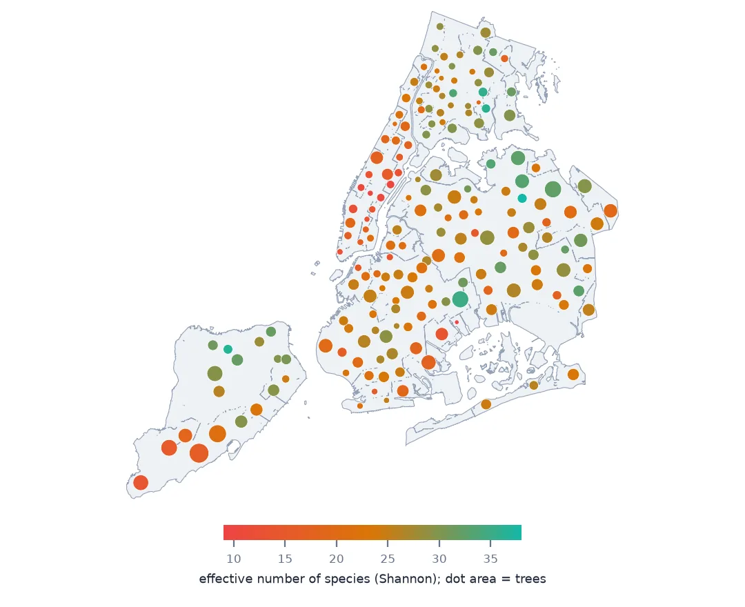
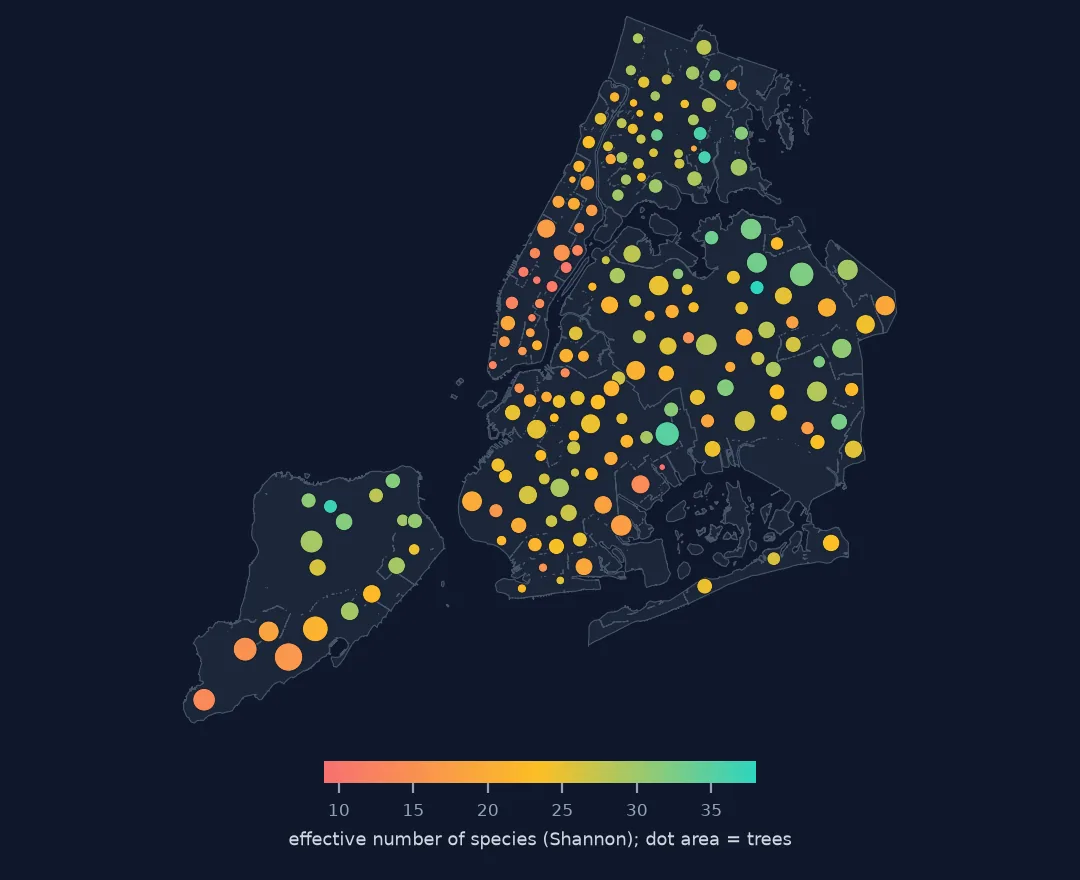
Across the 186 neighbourhoods with at least 500 trees, a median street-tree population is as diverse as 24.5 equally common species. The range is fourfold: Starrett City, where one species is 32% of the trees, is equivalent to 9.3 species; East Flushing to 38.0, with no species above 11%. Midtown is near the bottom, its 1,120 trees dominated by a few tolerant species.
Richness, indices and planting rules
1. Richness depends on how many trees you count
print(f"correlation of species count and tree count across neighbourhoods: {nta.species.corr(nta.trees, method='spearman'):.2f}")
rng = np.random.default_rng(0)
rare = {}
for name, g in alive.groupby("nta_name"):
    if len(g) >= 2000:
        rare[name] = len(set(rng.choice(g.spc_common.values, 1000, replace=False)))
rare = pd.Series(rare)
print(f"species in a random 1,000 trees: median {rare.median():.0f}, range {rare.min()}-{rare.max()}")
correlation of species count and tree count across neighbourhoods: 0.85
species in a random 1,000 trees: median 68, range 35-89
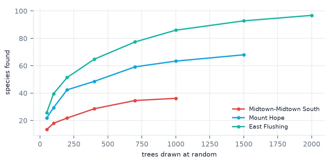
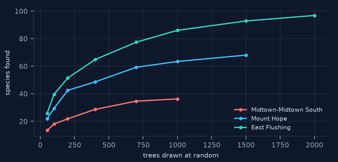
The raw species count tracks the number of trees closely (rank correlation 0.85): a neighbourhood with more trees will list more species whatever its diversity. Rarefaction removes that by drawing the same number of trees from each — in a random 1,000 trees the median neighbourhood has 68 species, from 35 to 89.
2. Shannon and Simpson weigh common species differently
nta["simpson"] = alive.groupby("nta_name").spc_common.apply(lambda s: 1 / (s.value_counts(normalize=True) ** 2).sum()).reindex(nta.index)
print(nta[["effective_species", "simpson"]].corr(method="spearman").round(2).to_string())
print(nta[["effective_species", "simpson"]].describe().round(1).to_string())
effective_species simpson
effective_species 1.00 0.94
simpson 0.94 1.00
effective_species simpson
count 186.0 186.0
mean 23.8 13.8
std 5.8 4.0
min 9.3 4.7
25% 19.9 11.2
50% 24.5 13.8
75% 28.1 16.5
max 38.0 23.0
Shannon and Simpson diversity rank neighbourhoods almost identically (0.94), but Simpson's effective number is lower — a median of 13.8 against 24.5 — because it weighs common species more. Reporting a single "diversity" without naming the index invites comparing numbers that are not comparable.
3. The 10-20-30 rule
genus = alive.spc_latin.str.split().str[0]
city_sp = alive.spc_common.value_counts(normalize=True)
city_gen = genus.value_counts(normalize=True)
print(f"city: largest species {city_sp.index[0]} {city_sp.iloc[0]:.1%}; largest genus {city_gen.index[0]} {city_gen.iloc[0]:.1%}")
over = alive.assign(genus=genus).groupby("nta_name").agg(sp=("spc_common", lambda s: s.value_counts(normalize=True).iloc[0]),
                                                        gen=("genus", lambda s: s.value_counts(normalize=True).iloc[0])).loc[nta.index]
print(f"neighbourhoods breaking 10% for one species: {(over.sp > 0.10).mean():.0%}; 20% for one genus: {(over.gen > 0.20).mean():.0%}")
city: largest species London planetree 13.3%; largest genus Acer 13.6%
neighbourhoods breaking 10% for one species: 97%; 20% for one genus: 48%
The 10-20-30 rule asks that no species exceed 10% of the trees, no genus 20% and no family 30%. Citywide the London planetree is 13.3% and the maples (Acer) 13.6%, so the city breaks the species limit and meets the genus one. Neighbourhoods do far worse: 97% have a species above 10%, and 48% have a genus above 20%.
4. Which species dominate where
dom = alive.groupby("nta_name").spc_common.agg(lambda s: s.value_counts().index[0]).loc[nta.index]
print(dom.value_counts().to_string())
spc_common
London planetree 80
honeylocust 63
pin oak 21
Callery pear 13
Norway maple 5
cherry 2
Japanese zelkova 1
littleleaf linden 1
Two species are the most common tree in most neighbourhoods: the London planetree in 80 and the honeylocust in 63. Pin oak leads in 21, Callery pear in 13 — mostly on Staten Island — and Norway maple still in 5.
Boroughs and generations
The data used on this page
New York City Department of Parks and Recreation, TreesCount! 2015 Street Tree Census on NYC Open Data: one row for every street tree, stump and dead tree mapped by staff and volunteers in 2015–2016, with species, trunk diameter, health and site conditions.
from pathlib import Path

import numpy as np
import pandas as pd
import requests

Path("data").mkdir(exist_ok=True)
SOCRATA = "https://data.cityofnewyork.us/api/views/{}/rows.csv?accessType=DOWNLOAD"
f = Path("data/nyc-street-tree-census-2015.csv")
if not f.exists():
    # TreesCount! 2015, the finished census (220 MB), NYC Open Data dataset uvpi-gqnh
    f.write_bytes(requests.get(SOCRATA.format("uvpi-gqnh"), timeout=1800).content)
trees = pd.read_csv(f, low_memory=False)
print(f"{len(trees):,} trees, {trees.status.eq('Alive').sum():,} alive")
683,788 trees, 652,173 alive
Example 1: diversity by borough
bor = alive.groupby("borough").spc_common.agg(lambda s: np.exp(shannon(s))).round(1)
print(bor.to_string())
borough
Bronx 33.7
Brooklyn 27.0
Manhattan 19.1
Queens 30.0
Staten Island 26.3
The Bronx's street trees are the most diverse, equivalent to 33.7 species, and Manhattan's the least, 19.1.
Example 2: new plantings are more diverse
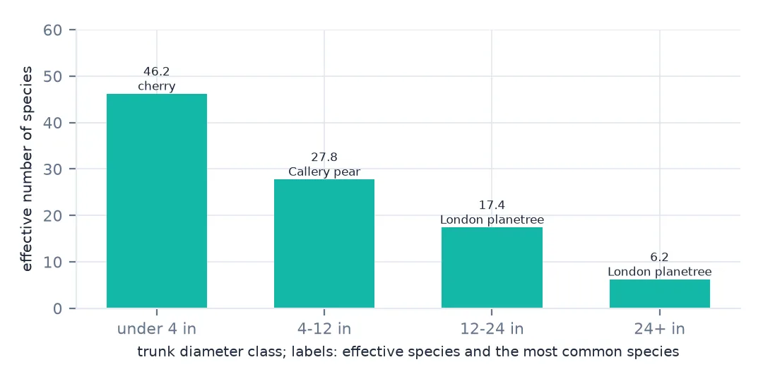
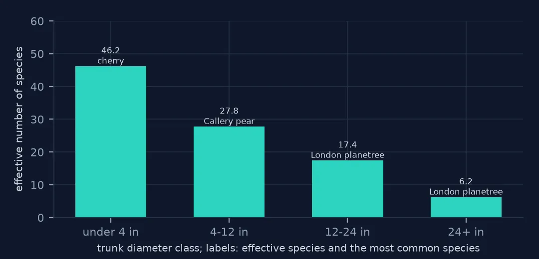
size = pd.cut(alive.tree_dbh, [0, 4, 12, 24, 500], labels=["under 4 in", "4-12 in", "12-24 in", "24+ in"])
print(alive.groupby(size, observed=True).spc_common.agg(lambda s: np.exp(shannon(s))).round(1).to_string())
print(alive.groupby(size, observed=True).spc_common.agg(lambda s: s.value_counts().index[0]).to_string())
tree_dbh
under 4 in 46.2
4-12 in 27.8
12-24 in 17.4
24+ in 6.2
tree_dbh
under 4 in cherry
4-12 in Callery pear
12-24 in London planetree
24+ in London planetree
The young trees are the most diverse: trees under 4 inches across, the most recently planted, are equivalent to 46.2 species, against 6.2 for trees over 24 inches. The large trees are dominated by the London planetree; the youngest by cherries. The street forest is diversifying from the bottom up.
Diversity as insurance
The point of measuring diversity is risk: the share of the forest that one pest or disease could remove. That is why foresters favour shares of the most common species and genus — the 10-20-30 rule — over indices: a 13% share of planetrees says directly what is at stake if a planetree disease arrives. Indices summarise the whole distribution and are better for comparing places, provided the index is named and the sample size is controlled.
Effective numbers make indices readable. A raw Shannon index means little; "as diverse as 24.5 equally common species" can be compared with the number of species present and with another neighbourhood's figure. Rarefaction does the same for richness, by asking how many species a fixed number of trees contains, which removes the advantage of simply having more trees.
Pitfalls in diversity measures
- Richness depends on sample size. Rarefy, or use an index.
- Name the index. Shannon and Simpson effective numbers differ by a factor of almost two here.
- Small neighbourhoods are noisy. A 500-tree threshold keeps 186 neighbourhoods.
- Common names hide genera. Use the Latin name's first word for the genus rule.
- "cherry" lumps several species in the census; diversity is a lower bound where names are coarse.
Internal links
- How to analyse New York's street tree census — the data
- How to compare two street tree censuses — how the species mix changed
- How to build a species richness grid from GBIF — richness with sampling effort in the wild
- Neighbourhood codes that match no boundary — the neighbourhood field
FAQ
How diverse are New York's street trees?
By neighbourhood, a median equivalent to 24.5 equally common species (Shannon), from 9.3 in Starrett City to 38.0 in East Flushing.
What is the 10-20-30 rule for street trees?
A planting guideline: no species above 10% of trees, no genus above 20%, no family above 30%. In 2015, 97% of New York's neighbourhoods had a species above 10%.