
How to Map Toxic Release Facilities by Amount Released
On this page
Problem statement
A map of toxic release facilities is easy to draw, a dot per facility from the coordinates in the Toxics Release Inventory, and hard to read: there are more than twenty thousand of them, and their releases range from a fraction of a pound to hundreds of millions of pounds. Sizing the dots by amount fixes the first problem and creates another, because a handful of mines would cover the map. This page totals each facility's 2024 releases, scales symbols on a log scale, colours them by industry and checks the points that overlap.
Quick answer
Total the facility's chemicals in pounds and make points from its coordinates:
t24["lb"] = pounds(t24)
fac = t24.groupby("TRIFD").agg(name=("FACILITY NAME", "first"), st=("ST", "first"), lb=("lb", "sum"),
                                lat=("LATITUDE", "first"), lon=("LONGITUDE", "first"), sector=("INDUSTRY SECTOR", "first"))
g = gpd.GeoDataFrame(fac, geometry=gpd.points_from_xy(fac.lon, fac.lat), crs=4269)
print(g.nlargest(5, "lb")[["name", "st", "sector", "lb"]].assign(lb=lambda d: (d.lb / 1e6).round(1)).to_string())
name st sector lb
TRIFD
99752RDDGP90MIL RED DOG OPERATIONS AK Metal Mining 723.9
84006KNNCT12300 KENNECOTT UTAH COPPER MINE CONCENTRATORS & POWER PLANT UT Metal Mining 192.7
99801KNNCT13401 HECLA GREENS CREEK MINING CO AK Metal Mining 87.6
7973WMDWYG8824F MIDWAY GAS PLANT TX Natural Gas Processing 73.3
85235SRCNC64ASA ASARCO LLC RAY COMPLEX/ HAYDEN SMELTER & CONCENTRATOR AZ Primary Metals 55.0
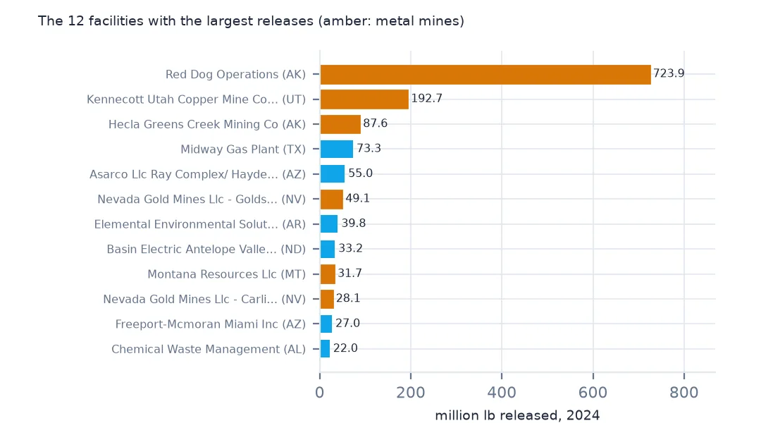
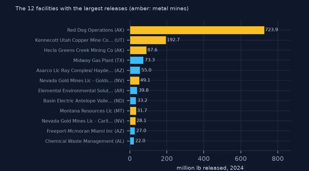
The largest are mines: Red Dog in Alaska released 723.9 million lb in 2024, Kennecott's Utah copper operations 192.7 million and Greens Creek in Alaska 87.6 million. A gas plant in Texas and a copper smelter in Arizona complete the top five.
Scaling circles to pounds
1. A range of eleven orders of magnitude
pos = g[g.lb > 0].lb
print(f"facilities releasing something: {len(pos):,}; smallest {pos.min():.4f} lb, median {pos.median():,.0f} lb, largest {pos.max():,.0f} lb")
facilities releasing something: 17,378; smallest 0.0000 lb, median 1,696 lb, largest 723,889,153 lb
17,378 facilities released something, from less than a ten-thousandth of a pound to 723,889,153 lb; the median is 1,696 lb. Proportional symbols on a linear scale would show one circle and a scatter of dots.
2. Circles by area, on a log scale
g["size"] = (np.log10(g.lb.clip(lower=1)) + 1) * 1.5
print(pd.cut(g.lb, [-1, 0, 1e3, 1e5, 1e6, 1e7, 1e9], labels=["0", "≤1k", "1k-100k", "100k-1M", "1M-10M", "10M+"]).value_counts(sort=False).to_string())
lb
0 4104
≤1k 7894
1k-100k 7686
100k-1M 1393
1M-10M 366
10M+ 39
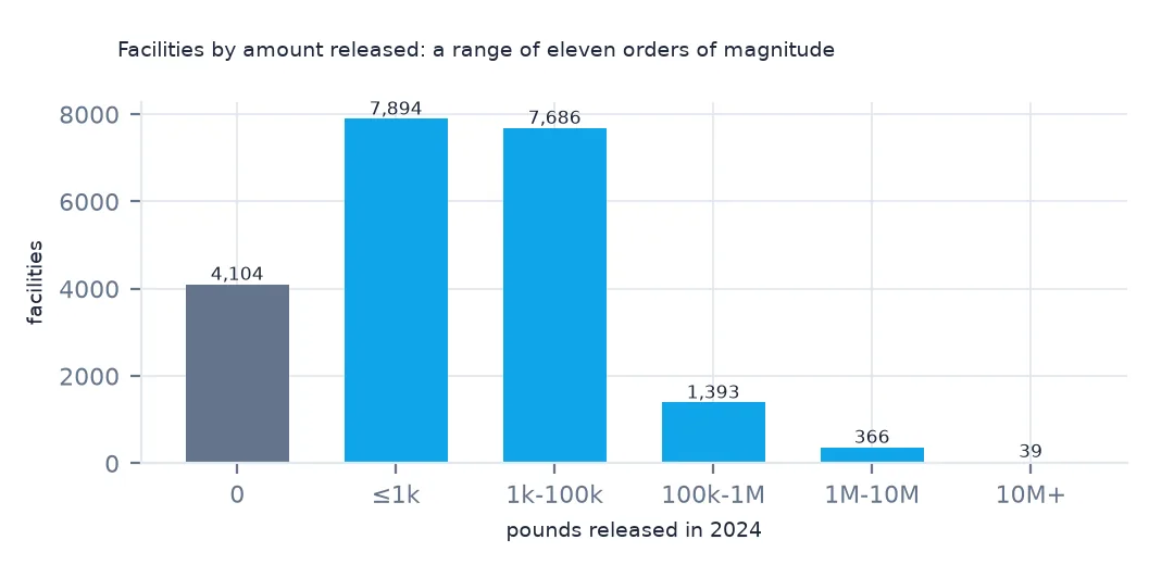
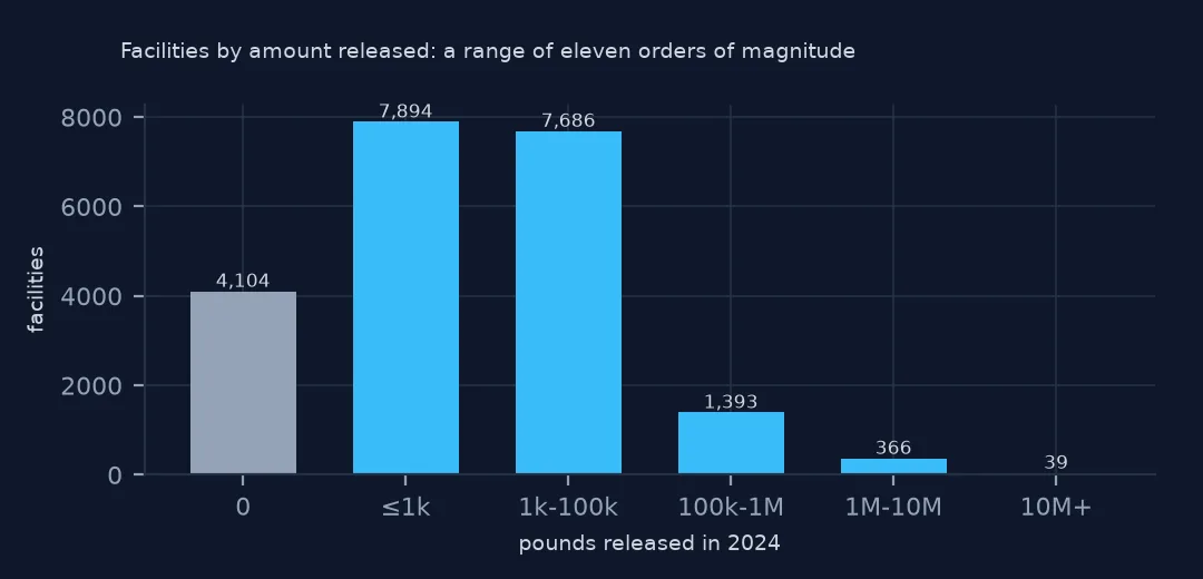
On a log scale the classes are usable: 7,894 facilities fall in the ≤1k lb class, 7,686 in 1k-100k, and 39 released more than 10 million lb. The 4,104 that released nothing get the smallest symbol rather than disappearing.
3. Facilities that sit on top of each other
dup = g.groupby(["lat", "lon"]).size()
print(f"locations shared by 2+ facilities: {(dup > 1).sum():,}, holding {dup[dup > 1].sum():,} facilities")
locations shared by 2+ facilities: 213, holding 472 facilities
213 locations hold two or more facilities, 472 in all. Sites with several operators report separately under one address, and their symbols stack.
By sector and by county
The data used on this page
The US EPA's Toxics Release Inventory basic data files for 2014 and 2024, public domain, downloaded on 16 October 2026 and saved on this site, because EPA revises past years when facilities resubmit. With them come the Census Bureau's Vintage 2025 county population estimates and 2024 county boundaries.
from pathlib import Path
import re
import zipfile

import geopandas as gpd
import numpy as np
import pandas as pd
import requests

Path("data").mkdir(exist_ok=True)
# EPA Toxics Release Inventory basic data files, reporting years 2014 and 2024, all states, xz-compressed and
# otherwise unchanged; Census Vintage 2025 county estimates and 2024 cartographic boundary counties.
# Downloaded 16 October 2026 and saved here, because EPA revises past years.
# Live: https://data.epa.gov/efservice/downloads/tri/mv_tri_basic_download/2024_US/csv (and 2014_US)
ARCHIVE = "epa-tri-2014-2024-2026-10-16.zip"
if not Path(f"data/{ARCHIVE}").exists():
    Path(f"data/{ARCHIVE}").write_bytes(requests.get(f"https://data.spatialworkflow.io/{ARCHIVE}", timeout=600).content)
Z = zipfile.ZipFile(f"data/{ARCHIVE}")


def tri(year):
    """One year's TRI file: a row per facility and chemical, columns numbered '1. YEAR' to '122. ...'."""
    d = pd.read_csv(Z.open(f"tri_{year}_us.csv.xz"), compression="xz", dtype=str, low_memory=False)
    d.columns = [re.sub(r"^\d+\.\s*", "", c) for c in d.columns]
    amounts = list(d.columns[d.columns.get_loc("5.1 - FUGITIVE AIR"):d.columns.get_loc("8.8 - ONE-TIME RELEASE") + 1])
    d[amounts + ["LATITUDE", "LONGITUDE"]] = d[amounts + ["LATITUDE", "LONGITUDE"]].apply(pd.to_numeric, errors="coerce")
    return d


def pounds(d, col="TOTAL RELEASES"):
    """A quantity in pounds: dioxin and dioxin-like compounds are reported in grams."""
    return d[col].where(d["UNIT OF MEASURE"] == "Pounds", d[col] / 453.59237)


t24 = tri(2024)
pop = pd.read_csv(Z.open("co-est2025-alldata.csv"), encoding="latin-1", dtype={"STATE": str, "COUNTY": str})
pop = pop[pop.SUMLEV == 50].assign(GEOID=lambda p: p.STATE + p.COUNTY)
Path("data/cb_2024_us_county_20m.zip").write_bytes(Z.read("cb_2024_us_county_20m.zip"))
counties = gpd.read_file("data/cb_2024_us_county_20m.zip")
print(f"TRI 2024: {len(t24):,} facility-chemical rows from {t24.TRIFD.nunique():,} facilities; {pounds(t24).sum() / 1e9:.2f} billion lb released")
TRI 2024: 77,295 facility-chemical rows from 21,482 facilities; 3.29 billion lb released
Example 1: the map coloured by sector
low = g[~g.st.isin(["AK", "HI", "PR", "GU", "VI", "MP", "AS"])].to_crs(5070)
top = low.groupby("sector").lb.sum().nlargest(5).index
print(low.assign(sector=low.sector.where(low.sector.isin(top), "other")).groupby("sector").agg(facilities=("lb", "size"), mlb=("lb", lambda s: round(s.sum() / 1e6, 1))).to_string())
ax = low.plot(column=low.sector.where(low.sector.isin(top), "other"), markersize=low["size"], alpha=0.6, legend=True, figsize=(11, 6))
ax.set_axis_off()
facilities mlb
sector
Chemicals 3369 448.7
Electric Utilities 358 178.9
Hazardous Waste 217 204.4
Metal Mining 82 505.3
Primary Metals 1375 344.3
other 15874 762.0
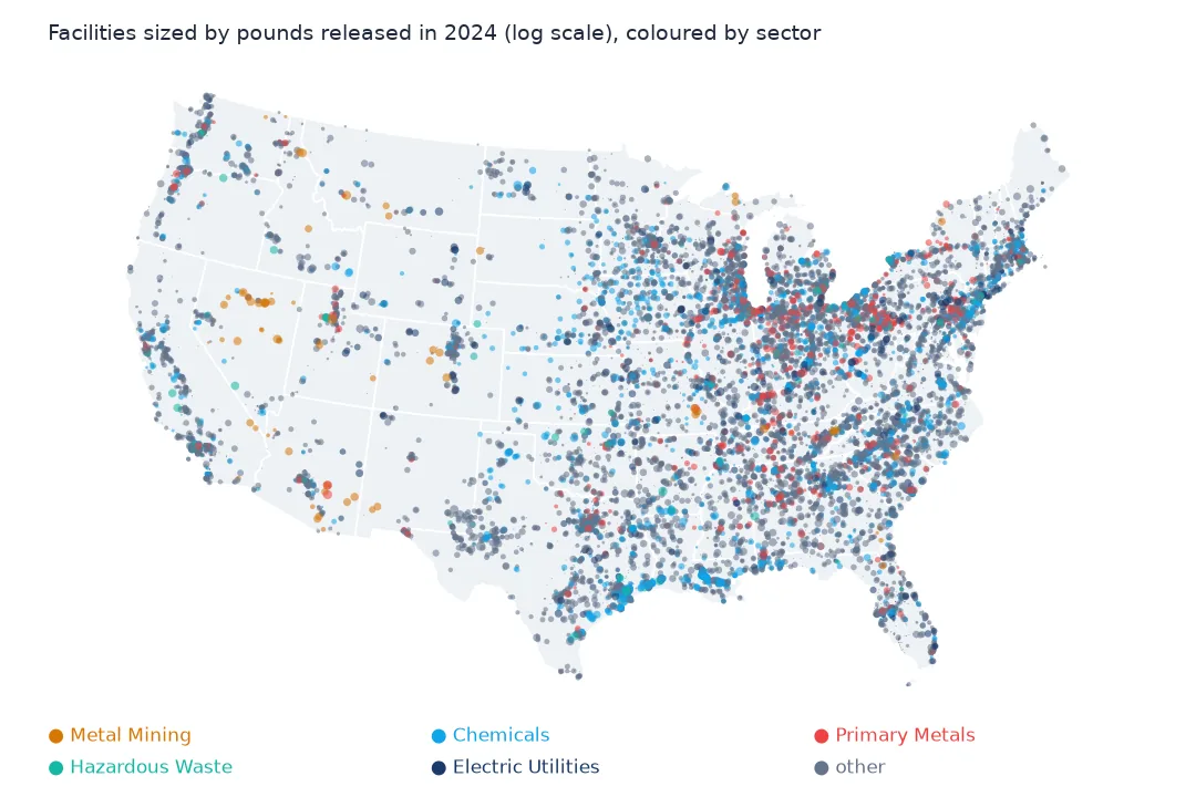
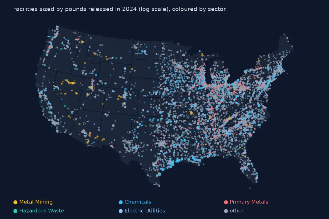
Chemical plants are the most numerous of the big five sectors, 3,369 facilities releasing 448.7 million lb, while 82 metal mines in the lower 48 released 505.3 million. Mines cluster in Nevada, Utah and Arizona, chemical plants along the Gulf Coast.
Example 2: counties with the most facilities
j = gpd.sjoin(g.to_crs(4269), counties.to_crs(4269)[["GEOID", "NAME", "STUSPS", "geometry"]], predicate="within")
print(j.groupby(["NAME", "STUSPS"]).size().nlargest(5).to_string())
NAME STUSPS
Harris TX 358
Los Angeles CA 307
Cook IL 290
Maricopa AZ 194
Cuyahoga OH 126
Harris County, Texas, home of the Houston Ship Channel, has the most facilities, 358, then Los Angeles and Cook counties.
Internal links
- Read the TRI files — the
tri()andpounds()helpers - The few facilities behind most releases — the largest circles, measured
- Air releases per resident — a map of what reaches the air
- County names — why this page joins counties by location