
How to Map Dams and High-Hazard Dams by County
On this page
Problem statement
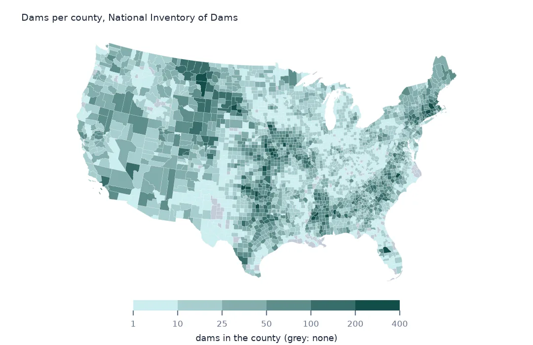
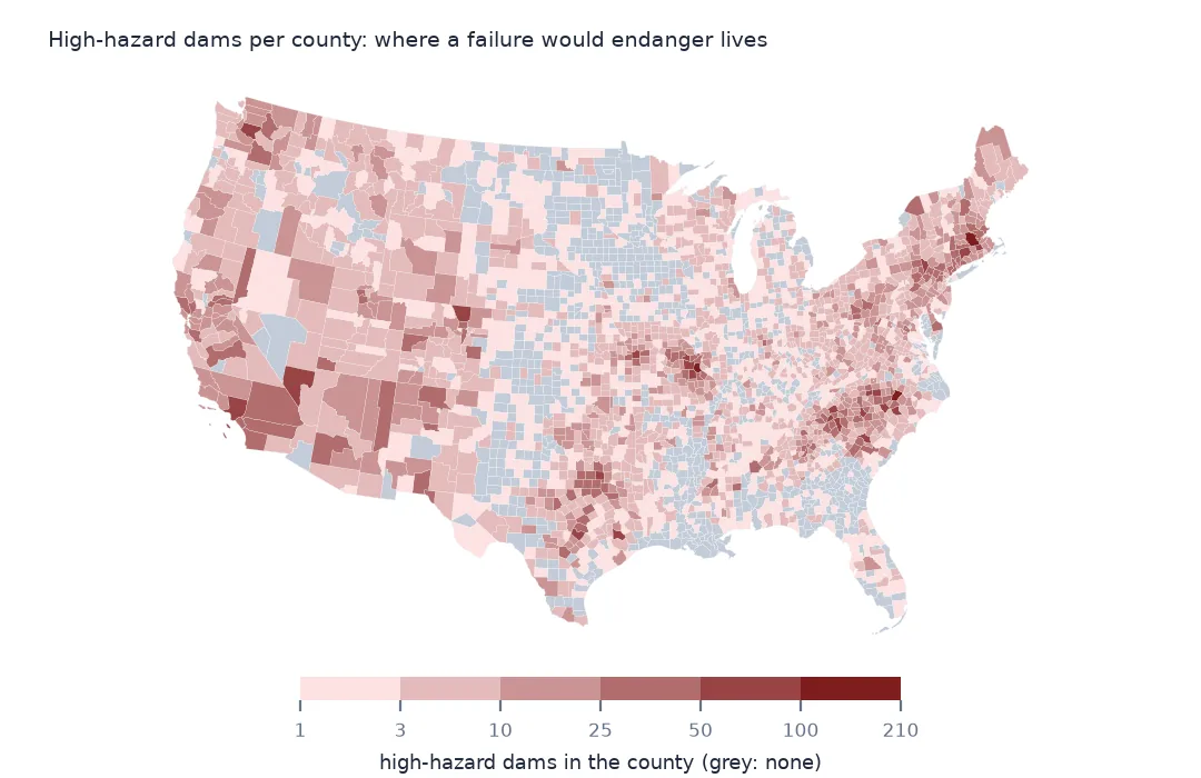
Some counties hold hundreds of dams, most of them small earthen dams on farm ponds and stock tanks; others have a handful of large ones. A county map of all dams shows where people have dammed small streams. A map of high-hazard dams shows where a failure would put lives at risk. Both maps start from the same join: the inventory's county column holds a county name, not a code, so the dams are placed in counties by their coordinates instead. This page counts dams per county both ways and maps them.
Quick answer
Join the dam points to the county polygons spatially, then count all dams and high-hazard dams per county:
dams = gpd.sjoin(nid[["nidId", "publicHazardId", "geometry"]], counties[["GEOID", "NAME", "STUSPS", "geometry"]].to_crs(nid.crs), predicate="within")
per = dams.groupby(["GEOID", "NAME", "STUSPS"]).agg(dams=("nidId", "size"), high=("publicHazardId", lambda s: (s == "High").sum())).reset_index()
print(per.nlargest(5, "dams").to_string(index=False))
print(per.nlargest(5, "high").to_string(index=False))
print(f"dams placed in a county: {len(dams):,} of {len(nid):,}; counties with a dam: {len(per):,}")
GEOID NAME STUSPS dams high
25027 Worcester MA 388 103
37183 Wake NC 363 207
20087 Jefferson KS 338 5
12105 Polk FL 325 19
19193 Woodbury IA 310 11
GEOID NAME STUSPS dams high
37183 Wake NC 363 207
25027 Worcester MA 388 103
29099 Jefferson MO 136 102
37119 Mecklenburg NC 156 89
29221 Washington MO 119 88
dams placed in a county: 92,595 of 92,626; counties with a dam: 3,041
Worcester County, Massachusetts, has the most dams in the inventory, 388, followed by Wake County, North Carolina, Jefferson County, Kansas, and Polk County, Florida. The high-hazard ranking is different. Wake County leads with 207 high-hazard dams, more than half its total, and Worcester is second with 103. Jefferson County, Kansas, has 338 dams but only 5 high hazard. 3,041 counties have at least one dam.
The join, checked
1. Why not join on the county column
names = nid.countyState.str.replace(" County", "", regex=False)
key = counties.NAME + ", " + counties.STATE_NAME
print(f"rows whose county name matches a 2024 county by name: {names.isin(key).mean():.1%}")
print(nid.loc[~names.isin(key), "countyState"].value_counts().head(4).to_string())
rows whose county name matches a 2024 county by name: 98.4%
countyState
Fairfield, Connecticut 220
Litchfield, Connecticut 220
New Haven, Connecticut 217
Hartford, Connecticut 171
A name join would work for 98.4% of rows. The failures are mostly Connecticut, whose dams still carry the eight historical counties, which the Census Bureau's 2024 boundaries replace with planning regions. A spatial join sidesteps names, spellings and boundary changes.
2. Dams outside every county
out = nid[~nid.nidId.isin(dams.nidId)]
print(f"outside the county polygons: {len(out)}; by state: {out.state.value_counts().head(4).to_dict()}")
outside the county polygons: 29; by state: {'Texas': 8, 'Virginia': 7, 'Michigan': 3, 'Wisconsin': 2}
31 rows, under 29 distinct ids, fall outside every county polygon. The 1:20 million county outlines are simplified, so a dam right at a shoreline or a state line can land just outside them. For exact counts use the 1:500,000 boundaries, or assign the stragglers to the nearest county with sjoin_nearest.
High-hazard density
The data used on this page
The US Army Corps of Engineers' National Inventory of Dams (NID), the whole inventory as a GeoPackage from its API, downloaded on 19 October 2026 and saved on this site, because the inventory is updated as states and agencies send revisions. Heights are in feet, storage in acre-feet and areas in acres, as the NID gives them.
from pathlib import Path
import zipfile

import geopandas as gpd
import numpy as np
import pandas as pd
import requests

Path("data").mkdir(exist_ok=True)
# US Army Corps of Engineers, National Inventory of Dams: the whole inventory as a GeoPackage, and the Census
# Bureau's 2024 cartographic boundary counties. Saved 19 October 2026, because the inventory is updated continuously.
# Live: https://nid.sec.usace.army.mil/api/nation/gpkg
ARCHIVE = "usace-nid-2026-10-19.zip"
if not Path(f"data/{ARCHIVE}").exists():
    Path(f"data/{ARCHIVE}").write_bytes(requests.get(f"https://data.spatialworkflow.io/{ARCHIVE}", timeout=900).content)
Z = zipfile.ZipFile(f"data/{ARCHIVE}")
if not Path("data/nid.gpkg").exists():
    Z.extract("nid.gpkg", "data")
NUMERIC = ["damHeight", "hydraulicHeight", "structuralHeight", "nidHeight", "damLength", "volume", "yearCompleted",
           "nidStorage", "maxStorage", "normalStorage", "surfaceArea", "drainageArea", "maxDischarge"]
nid = gpd.read_file("data/nid.gpkg")
nid[NUMERIC] = nid[NUMERIC].apply(pd.to_numeric, errors="coerce")       # the GeoPackage stores them as text
Path("data/cb_2024_us_county_20m.zip").write_bytes(Z.read("cb_2024_us_county_20m.zip"))
counties = gpd.read_file("data/cb_2024_us_county_20m.zip")
print(f"National Inventory of Dams: {len(nid):,} rows, {nid.nidId.nunique():,} NID ids; counties: {len(counties):,}")
National Inventory of Dams: 92,626 rows, 91,840 NID ids; counties: 3,222
Example 1: high-hazard dams per 1,000 km²
per = per.merge(counties[["GEOID", "ALAND"]], on="GEOID")
per["high_per_1000km2"] = per.high / per.ALAND * 1e9
print(per[per.high >= 10].nlargest(5, "high_per_1000km2")[["NAME", "STUSPS", "high", "high_per_1000km2"]].round(1).to_string(index=False))
NAME STUSPS high high_per_1000km2
Wake NC 207 95.8
Passaic NJ 46 95.4
Rockwall TX 26 78.9
Warren MO 78 70.3
Mecklenburg NC 89 65.6
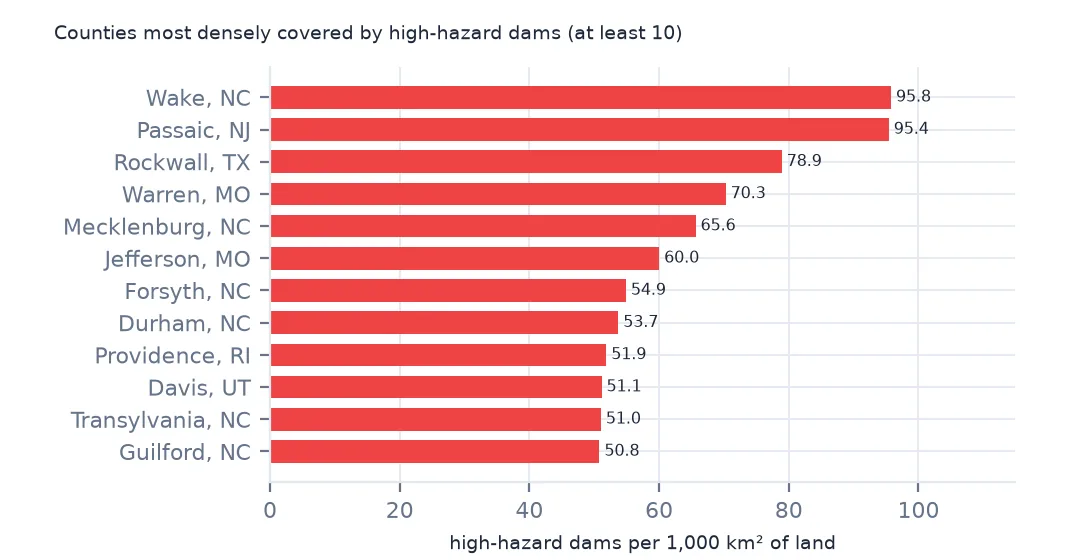
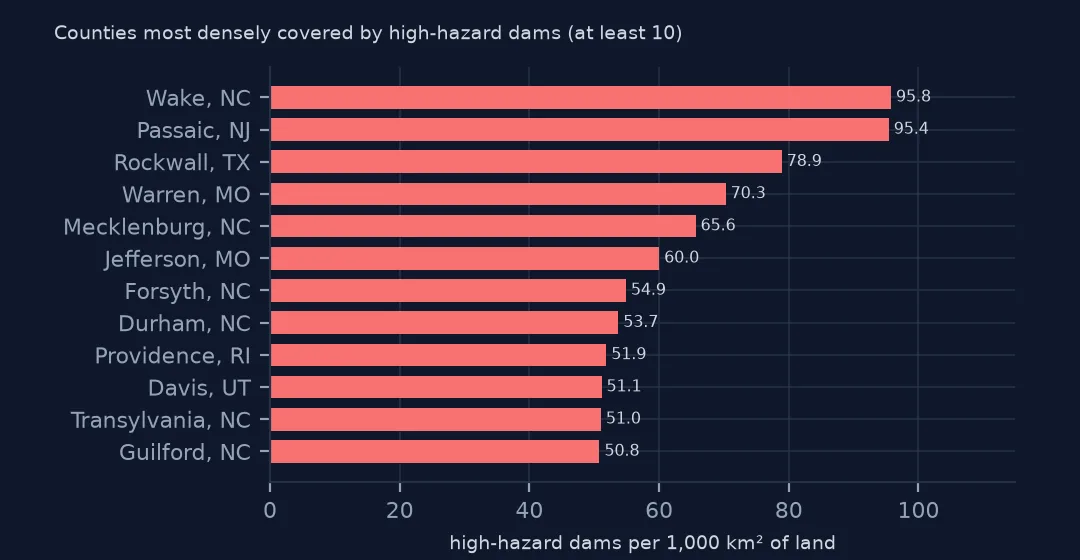
Among counties with at least ten high-hazard dams, Wake County again has the most per area, 95.8 per 1,000 km², closely followed by Passaic County, New Jersey. Rockwall in Texas, Warren in Missouri and Mecklenburg, home of Charlotte, follow. Most of them are fast-growing suburban counties, where houses now stand below dams that once had only fields downstream.
Example 2: the choropleth
m = counties.merge(per[["GEOID", "dams", "high"]], on="GEOID", how="left")
m = m[~m.STATEFP.isin(["02", "15", "60", "66", "69", "72", "78"])].to_crs(5070)
ax = m.plot(column="dams", scheme="FisherJenks", k=6, cmap="YlGnBu", legend=True, missing_kwds={"color": "#eeeeee"}, figsize=(11, 6))
ax.set_axis_off()
print(f"lower 48 counties with no dam in the inventory: {m.dams.isna().sum()}")
lower 48 counties with no dam in the inventory: 116
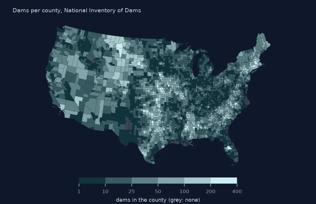
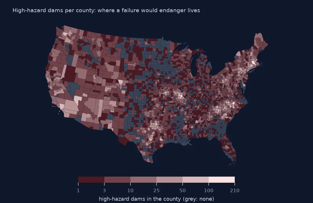
On the choropleth, the darkest counties are in the plains of Montana and the Dakotas, from north Texas to Kansas, across the Southeast and in New England. Only 116 counties in the lower 48 have no dam in the inventory at all. The high-hazard map looks different: its darkest counties are in the Piedmont of the Carolinas, the Ozarks of Missouri, southern New England and some large counties of California and Arizona.
Internal links
- Hazard potential explained — what the high-hazard map shows and doesn't
- High-hazard dams in poor condition — the dams to watch, by state
- Reading the inventory — the columns
- Bridges in poor condition by county — the same county count for bridges