
How to extract a Sentinel-1 time series for an area
On this page
Problem statement
A single radar image says how bright a surface is; a time series says what it is doing. Rice paddies drown and drain, cereals grow and are cut, reservoirs rise and fall, and each leaves a shape in backscatter that a single date cannot show. Building that series from a catalogue is where the work is: the frames have to be grouped into passes, the passes kept to one relative orbit, the values averaged over the area in linear units, and the result labelled with enough metadata to be reproducible.
Over a block of rice fields near Sueca, south of the Albufera, a year of Sentinel-1 VV from one descending orbit runs from −17.4 dB when the fields are under water to −7.0 dB at the height of the canopy: a ten-decibel swing, measured every twelve days through a season when optical imagery is repeatedly lost to cloud.
Quick answer
Group into passes, keep one orbit, and average linear values inside the polygon:
import numpy as np, pandas as pd, geopandas as gpd
from rasterio.features import geometry_mask
from sar_io import search, passes, grid, read_pass, to_db

bbox = [-0.345, 39.255, -0.300, 39.285]             # rice fields near Sueca, south of the Albufera
g = grid(bbox, "EPSG:25830")
area = gpd.GeoSeries.from_wkt(
    ["POLYGON((-0.334 39.262, -0.313 39.262, -0.313 39.278, -0.334 39.278, -0.334 39.262))"],
    crs=4326).to_crs(g["crs"])
inside = ~geometry_mask(area, out_shape=(g["height"], g["width"]),
                        transform=g["transform"], invert=False)

rows = []
for (day, orbit), frames in passes(search(bbox, "2024-01-01/2024-12-31", orbit=110)).items():
    vv, vh = read_pass(frames, "vv", g), read_pass(frames, "vh", g)
    rows.append({"date": pd.Timestamp(day), "orbit": orbit,
                 "vv_db": to_db(np.nanmean(vv[inside])), "vh_db": to_db(np.nanmean(vh[inside])),
                 "pixels": int(np.isfinite(vv[inside]).sum())})
ts = pd.DataFrame(rows).set_index("date")
print(f"{len(ts)} passes; VV from {ts.vv_db.min():.1f} to {ts.vv_db.max():.1f} dB")
print(ts.head(3).round(2).to_string())
26 passes; VV from -17.4 to -7.0 dB
orbit vv_db vh_db pixels
date
2024-01-06 110 -11.80 -21.590000 32214
2024-01-18 110 -12.68 -21.639999 32214
2024-02-23 110 -8.59 -18.209999 32214
Averaging inside the polygon in linear units and converting once at the end is what keeps the series comparable with published figures.
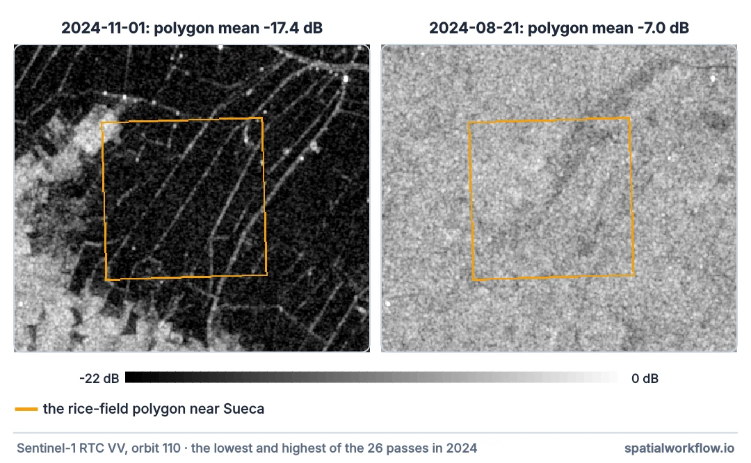
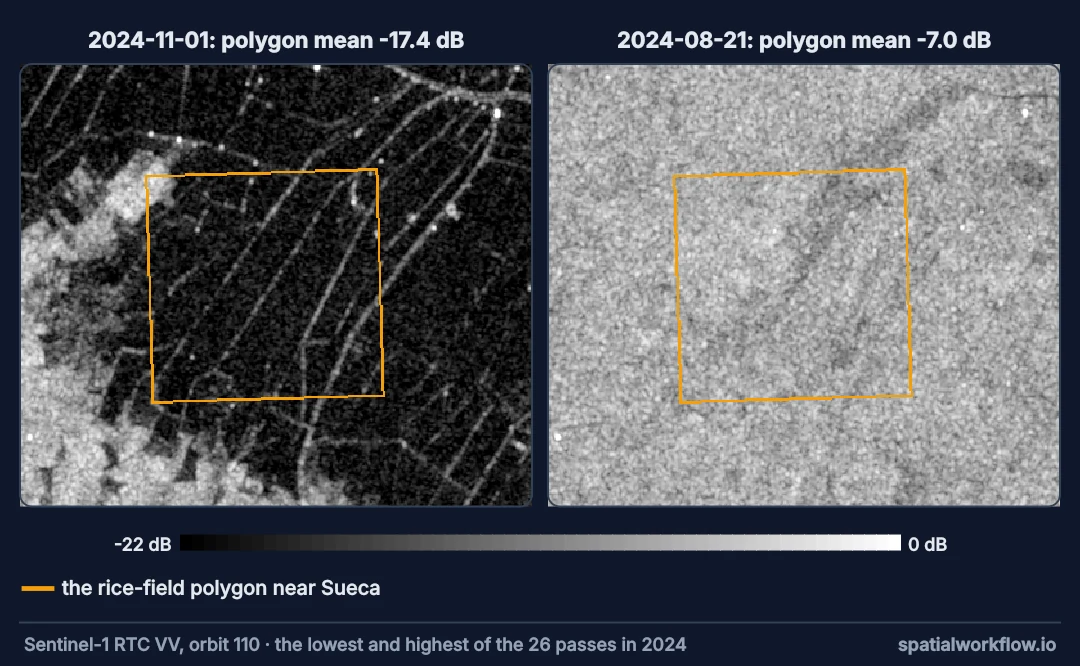
A grid around the polygon, one orbit, linear means
1. Choose the polygon and a grid around it
Read onto a grid covering the polygon's bounding box, with a small margin, so every pass lands on the same pixels.
2. Keep to one relative orbit
Different orbits differ by a decibel or more on the same surface. Mixing them puts a sawtooth in the series that looks like a signal.
3. Average in linear power
Take the mean of linear values inside the polygon, then convert to decibels once, as the decibel guide explains.
4. Record the pixel count
A pass whose frames cover only part of the polygon gives a mean over fewer pixels. Store the count and drop passes far below the usual.
5. Keep both polarisations and the ratio
VV responds to surface and water, VH to canopy volume. Their ratio often separates growth stages better than either.
6. Interpret with a calendar
Radar sees structure and water, not crop type. A curve becomes an interpretation only alongside what is known about the local cropping calendar.
A year of backscatter over rice fields
The data used on this page
Sentinel-1 radiometrically terrain-corrected backscatter (sentinel-1-rtc) from the Microsoft Planetary Computer, read through sar_io.py — the small module from the reading guide that searches, groups frames into passes and mosaics each pass onto a fixed grid.
%%writefile sar_io.py
"""Find, read and mosaic Sentinel-1 RTC scenes from Microsoft Planetary Computer."""
from collections import defaultdict

import numpy as np
import planetary_computer
import pystac_client
import rasterio
from rasterio.enums import Resampling
from rasterio.transform import from_origin
from rasterio.vrt import WarpedVRT
from rasterio.warp import transform_bounds

STAC = "https://planetarycomputer.microsoft.com/api/stac/v1"


def search(bbox, dates, orbit=None, direction=None, collection="sentinel-1-rtc"):
    """Items over bbox (lon/lat) in a date range, filtered by relative orbit and pass direction."""
    cat = pystac_client.Client.open(STAC, modifier=planetary_computer.sign_inplace)
    items = cat.search(collections=[collection], bbox=bbox, datetime=dates).item_collection()
    keep = [i for i in items
            if (orbit is None or i.properties["sat:relative_orbit"] == orbit)
            and (direction is None or i.properties["sat:orbit_state"] == direction)]
    return sorted(keep, key=lambda i: i.datetime)


def passes(items):
    """Group frames into passes: same day, same relative orbit."""
    groups = defaultdict(list)
    for i in items:
        groups[(i.datetime.date(), i.properties["sat:relative_orbit"])].append(i)
    return dict(sorted(groups.items()))


def grid(bbox, crs, res=10):
    """A fixed target grid: every pass is read onto this, so arrays line up."""
    left, bottom, right, top = transform_bounds(4326, crs, *bbox)
    width, height = int((right - left) // res), int((top - bottom) // res)
    return {"crs": crs, "transform": from_origin(left, top, res, res),
            "width": width, "height": height}


def read_pass(frames, band, g):
    """Mosaic one pass's frames for one band onto grid g. Linear power; NaN where no data."""
    out = np.full((g["height"], g["width"]), np.nan, dtype="float32")
    for item in frames:
        with rasterio.open(item.assets[band].href) as src, WarpedVRT(
                src, crs=g["crs"], transform=g["transform"], width=g["width"],
                height=g["height"], resampling=Resampling.bilinear, nodata=np.nan) as vrt:
            a = vrt.read(1)
        a[a <= 0] = np.nan                       # -32768 nodata and zero-padding
        fill = np.isnan(out) & np.isfinite(a)
        out[fill] = a[fill]
    return out


def to_db(linear):
    return 10 * np.log10(linear)
Overwriting sar_io.py
Example 1 — the shape of the year
monthly = ts.resample("MS").mean(numeric_only=True)
for month, row in monthly.iterrows():
    bar = "#" * int((row.vv_db + 20) * 2)
    print(f"{month:%Y-%m}  VV {row.vv_db:6.1f} dB  VH {row.vh_db:6.1f} dB  {bar}")
2024-01 VV -12.2 dB VH -21.6 dB ###############
2024-02 VV -8.6 dB VH -18.2 dB ######################
2024-03 VV -9.0 dB VH -18.4 dB ######################
2024-04 VV -9.7 dB VH -18.3 dB ####################
2024-05 VV -13.1 dB VH -21.3 dB #############
2024-06 VV -10.2 dB VH -19.0 dB ###################
2024-07 VV -8.6 dB VH -17.1 dB ######################
2024-08 VV -7.9 dB VH -14.6 dB ########################
2024-09 VV -7.9 dB VH -15.2 dB ########################
2024-10 VV -9.0 dB VH -16.2 dB ######################
2024-11 VV -14.8 dB VH -23.2 dB ##########
2024-12 VV -9.5 dB VH -19.6 dB ####################
The monthly means trace the paddy calendar: dips in May and November, when the fields are deliberately flooded, and a peak in August and September, when the canopy is at its fullest. In monthly means VH swings further than VV, 8.6 dB against 6.9, because the canopy depolarises; over individual passes both span about 10.5 dB.
Example 2 — why one orbit only
month = passes(search(bbox, "2024-07-01/2024-07-31"))
for (day, orbit), frames in month.items():
    vv = read_pass(frames, "vv", g)
    print(f"{day} orbit {orbit:3d} {frames[0].properties['sat:orbit_state']:10} "
          f"VV {to_db(np.nanmean(vv[inside])):6.2f} dB")
2024-07-03 orbit 103 ascending VV -8.34 dB
2024-07-04 orbit 110 descending VV -8.08 dB
2024-07-09 orbit 8 descending VV -9.95 dB
2024-07-10 orbit 30 ascending VV -9.65 dB
2024-07-15 orbit 103 ascending VV -8.51 dB
2024-07-16 orbit 110 descending VV -8.42 dB
2024-07-22 orbit 30 ascending VV -8.76 dB
2024-07-27 orbit 103 ascending VV -8.78 dB
2024-07-28 orbit 110 descending VV -9.17 dB
Example 3 — save it with its provenance
ts["vh_vv_db"] = ts.vh_db - ts.vv_db
ts.attrs = {"collection": "sentinel-1-rtc", "relative_orbit": 110, "polygon_crs": str(g["crs"]),
            "statistic": "mean of linear gamma0 inside the polygon, converted to dB"}
ts.round(3).to_csv("rice_vv_vh_2024_orbit110.csv")
print(ts[["vv_db", "vh_db", "vh_vv_db", "pixels"]].describe().round(2).to_string())
vv_db vh_db vh_vv_db pixels
count 26.00 26.00 26.00 26.0
mean -9.91 -18.39 -8.49 32214.0
std 2.44 2.86 1.32 0.0
min -17.41 -24.41 -11.19 32214.0
25% -10.03 -19.65 -9.55 32214.0
50% -9.19 -18.29 -8.67 32214.0
75% -8.47 -15.91 -7.30 32214.0
max -7.05 -13.65 -6.55 32214.0
Rice as the clearest example
Why rice is the clearest example
A flooded paddy is a mirror: much of the pulse is reflected away, and VV drops towards the values of open water. As the crop grows, stems and leaves scatter, and both channels rise — VH fastest, because the canopy depolarises. When the fields are drained and cut, the series falls again. Few land covers move through such a wide range in a year, which is why rice mapping was one of the first operational uses of radar.
Why the mean, and what it hides
The mean over a polygon is a convenient summary; it is also blind to the difference between all fields changing a little and a few changing a lot. Keeping a percentile or two — the 10th and 90th within the polygon — costs nothing and shows whether the fields are moving together.
Why the series still needs the metadata
Backscatter has no absolute meaning without the geometry it was measured in. A published series that does not state the collection, the orbit, the polarisation, the statistic and the polygon cannot be compared with any other — and cannot be reproduced next year by its own author.
Partial coverage, wind and mixed polygons
- Partial coverage gives a mean over part of the polygon; track the pixel count.
- Wind on flooded fields raises VV by several decibels for one date.
- Mixed polygons — half rice, half orchard — average into a curve that describes neither.
- Border pixels mix in roads and canals; erode the polygon by a pixel or two.
- Sentinel-1C adds passes from 2025; a series crossing that boundary changes sampling rate.
- Coherence time series from SLC add information intensity does not carry.
Internal links
- How to find Sentinel-1 scenes in Python — passes and orbits
- How to convert SAR backscatter to decibels — averaging correctly
- SAR polarisation explained — what VV and VH each track
- How to monitor crops with Sentinel-1 in Python — using the ratio
- How to extract an NDVI time series for a polygon — the optical counterpart
- How to calculate zonal statistics in Python — polygon means in general
FAQ
How do I build a Sentinel-1 time series for a field?
Search the RTC collection, group frames into passes, keep one relative orbit, and average linear backscatter inside the polygon per pass.
Why must I keep to one orbit?
Different orbits have different look directions and incidence angles, which shifts backscatter by a decibel or more.
Should I average in dB?
No. Average linear values and convert the mean.
How often do I get a value?
Every 12 days per orbit with one satellite; more often if you accept several orbits as separate series.
What does a drop of 10 dB mean over farmland?
Usually flooding or irrigation; a drop that large is water appearing.
Can I compare my curve with a published one?
Only if both state collection, orbit, polarisation and statistic.