How to monitor crops with Sentinel-1 in Python

On this page

Problem statement

Radar monitors crops through the cloudy half of the year, when optical indices go missing for weeks. What it measures is structure and water rather than greenness, so the workflow is different: instead of one index, you track two channels and their ratio; instead of a single date, you use the shape of the season; and instead of a threshold, you usually end up with a classifier trained on the features that separate the covers you care about.

On the fields south of Valencia, the VH/VV ratio of cropland rises from −8.2 dB in late winter to −6.9 dB at the height of summer, while built-up land sits between −8.3 and −8.6 dB all year. A classifier given three summer features — VV, VH and their ratio — reaches 71.6% recall on cropland and 68.8% on built-up land, and 0% on open water, for a reason worth more than the number itself.

Quick answer

Build a small feature stack from a seasonal composite and add the ratio:

import numpy as np
from sar_io import search, passes, grid, read_pass, to_db

bbox = [-0.46, 39.25, -0.33, 39.45]
g = grid(bbox, "EPSG:25830")

def composite(dates, band, orbit=110):
    stack = [read_pass(f, band, g) for f in passes(search(bbox, dates, orbit=orbit)).values()]
    return np.nanmean(np.stack(stack), axis=0)

summer = "2024-06-01/2024-09-15"
vv, vh = composite(summer, "vv"), composite(summer, "vh")
features = np.stack([to_db(vv), to_db(vh), to_db(vh) - to_db(vv)])
print("features:", ["VV dB", "VH dB", "VH/VV dB"], features.shape)
print("medians:", np.round(np.nanmedian(features, axis=(1, 2)), 2))

features: ['VV dB', 'VH dB', 'VH/VV dB'] (3, 2252, 1184)
medians: [ -9.16 -16.25  -6.94]

Three features from one composite: two channels and the ratio that says how much of the return came from volume scattering.

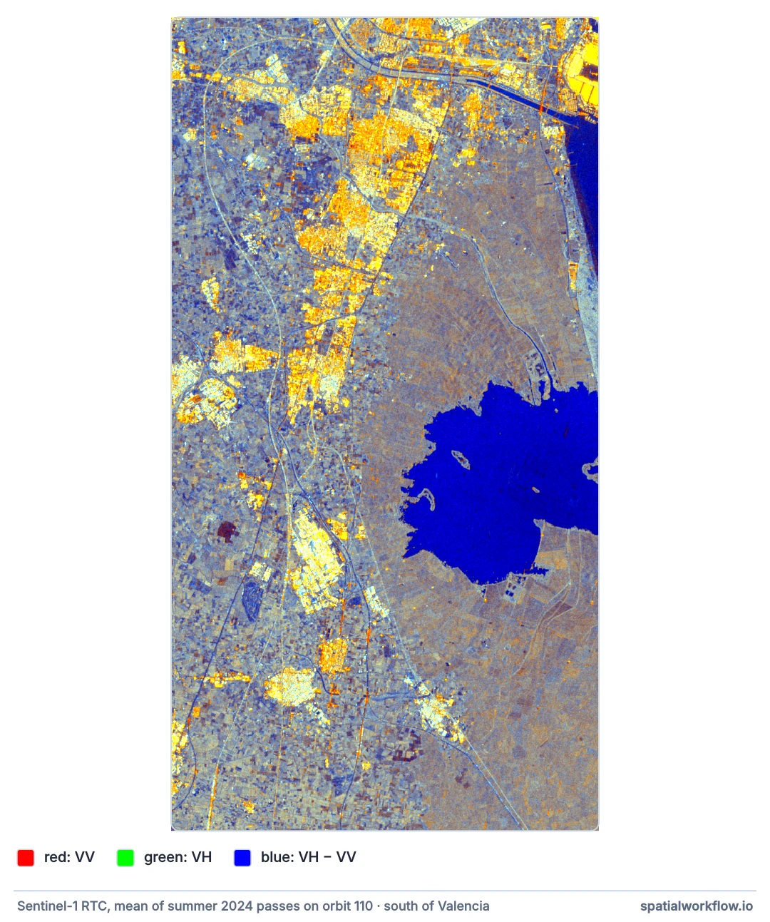
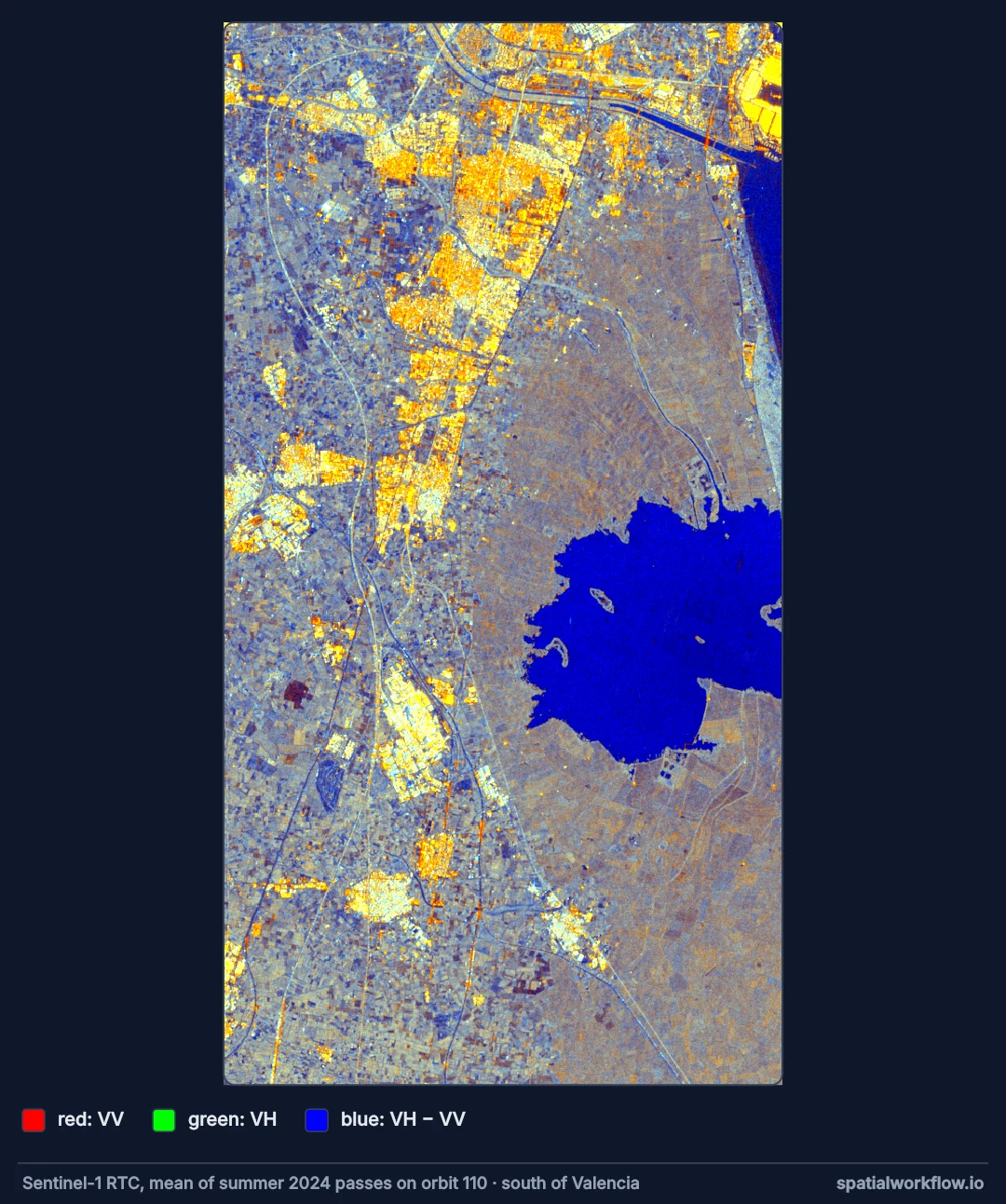
False-colour radar composite south of Valencia: towns bright yellow and orange, orchards and fields in mottled blue-grey, the rice fields around the lagoon in brownish grey, and the Albufera lagoon itself deep blue. — The three features as one false-colour image: VV in red, VH in green, the ratio in blue. Towns come out yellow-orange (strong VV and VH), the orchards on the western plain blue-grey, the rice fields around the lagoon a flatter brown, and open water deep blue, where almost nothing comes back but the ratio stays high. Land-cover classes that look alike in one band separate in three.

Cropland's ratio rises 1.3 dB from winter to summer; built-up land moves by a third of that.

Decide the separation, composite seasons, add the ratio

1. Decide what you are separating

Water from land is a one-feature problem. Vegetation from buildings is a two-feature problem. Crop type from crop type needs the whole season and usually more.

2. Composite a season, per orbit

Average the passes of one relative orbit over the period, in linear units. A season composite is much less noisy than a date, and it keeps full resolution.

3. Add the ratio

VH minus VV in decibels. It cancels much of what soil moisture and incidence angle do to both channels.

4. Use the seasonal shape when you can

Two composites — one early, one late — or monthly means per field are far more informative than one composite, because the trajectory separates covers that look alike on any single date.

5. Validate spatially

Train on one part of the scene and test on another, never on a random pixel split. Neighbouring pixels are nearly the same observation, and a random split reports an accuracy that will not transfer.

6. Treat reference maps as references, not truth

ESA WorldCover is itself a model with its own errors, and it describes 2021. Using it as labels measures agreement with it, which is not the same as accuracy.

Different pairs of classes need different features; no single channel separates everything.

Crop classes through the year

The data used on this page

Sentinel-1 radiometrically terrain-corrected backscatter (sentinel-1-rtc) from the Microsoft Planetary Computer, read through sar_io.py — the small module from the reading guide that searches, groups frames into passes and mosaics each pass onto a fixed grid.

%%writefile sar_io.py
"""Find, read and mosaic Sentinel-1 RTC scenes from Microsoft Planetary Computer."""
from collections import defaultdict

import numpy as np
import planetary_computer
import pystac_client
import rasterio
from rasterio.enums import Resampling
from rasterio.transform import from_origin
from rasterio.vrt import WarpedVRT
from rasterio.warp import transform_bounds

STAC = "https://planetarycomputer.microsoft.com/api/stac/v1"


def search(bbox, dates, orbit=None, direction=None, collection="sentinel-1-rtc"):
    """Items over bbox (lon/lat) in a date range, filtered by relative orbit and pass direction."""
    cat = pystac_client.Client.open(STAC, modifier=planetary_computer.sign_inplace)
    items = cat.search(collections=[collection], bbox=bbox, datetime=dates).item_collection()
    keep = [i for i in items
            if (orbit is None or i.properties["sat:relative_orbit"] == orbit)
            and (direction is None or i.properties["sat:orbit_state"] == direction)]
    return sorted(keep, key=lambda i: i.datetime)


def passes(items):
    """Group frames into passes: same day, same relative orbit."""
    groups = defaultdict(list)
    for i in items:
        groups[(i.datetime.date(), i.properties["sat:relative_orbit"])].append(i)
    return dict(sorted(groups.items()))


def grid(bbox, crs, res=10):
    """A fixed target grid: every pass is read onto this, so arrays line up."""
    left, bottom, right, top = transform_bounds(4326, crs, *bbox)
    width, height = int((right - left) // res), int((top - bottom) // res)
    return {"crs": crs, "transform": from_origin(left, top, res, res),
            "width": width, "height": height}


def read_pass(frames, band, g):
    """Mosaic one pass's frames for one band onto grid g. Linear power; NaN where no data."""
    out = np.full((g["height"], g["width"]), np.nan, dtype="float32")
    for item in frames:
        with rasterio.open(item.assets[band].href) as src, WarpedVRT(
                src, crs=g["crs"], transform=g["transform"], width=g["width"],
                height=g["height"], resampling=Resampling.bilinear, nodata=np.nan) as vrt:
            a = vrt.read(1)
        a[a <= 0] = np.nan                       # -32768 nodata and zero-padding
        fill = np.isnan(out) & np.isfinite(a)
        out[fill] = a[fill]
    return out


def to_db(linear):
    return 10 * np.log10(linear)

Overwriting sar_io.py

Example 1 — the ratio through the year, by class

import pystac_client, planetary_computer, rasterio
from rasterio.enums import Resampling
from rasterio.vrt import WarpedVRT

cat = pystac_client.Client.open("https://planetarycomputer.microsoft.com/api/stac/v1",
                                modifier=planetary_computer.sign_inplace)
wc_item = next(cat.search(collections=["esa-worldcover"], bbox=bbox).items())
with rasterio.open(wc_item.assets["map"].href) as src, WarpedVRT(
        src, crs=g["crs"], transform=g["transform"], width=g["width"], height=g["height"],
        resampling=Resampling.nearest) as vrt:
    wc = vrt.read(1)

classes = {40: "cropland", 10: "tree cover", 30: "grassland", 50: "built-up"}
print(f"{'period':12} " + " ".join(f"{n:>11}" for n in classes.values()))
for label, dates in [("Feb–Mar", "2024-02-01/2024-03-31"), ("May–Jun", "2024-05-01/2024-06-30"),
                     ("Jul–Aug", "2024-07-01/2024-08-31"), ("Oct–Nov", "2024-10-01/2024-11-30")]:
    r = to_db(composite(dates, "vh")) - to_db(composite(dates, "vv"))
    print(f"{label:12} " + " ".join(f"{np.nanmedian(r[wc == c]):11.2f}" for c in classes))

period          cropland  tree cover   grassland    built-up
Feb–Mar            -8.22       -6.59       -6.81       -8.52
May–Jun            -8.22       -6.46       -6.69       -8.35
Jul–Aug            -6.88       -6.33       -6.54       -8.30
Oct–Nov            -7.12       -6.45       -6.62       -8.64

Example 2 — which feature separates which pair

def separability(a, b):
    return abs(np.nanmedian(a) - np.nanmedian(b)) / np.nanstd(np.concatenate([a, b]))

names = ["VV", "VH", "VH/VV"]
for code, name in {10: "tree cover", 50: "built-up", 80: "open water"}.items():
    scores = [separability(f[wc == 40], f[wc == code]) for f in features]
    best = names[int(np.argmax(scores))]
    print(f"cropland vs {name:11} " + "  ".join(f"{n} {s:4.2f}" for n, s in zip(names, scores))
          + f"   best: {best}")

cropland vs tree cover  VV 0.09  VH 0.64  VH/VV 0.59   best: VH
cropland vs built-up    VV 1.19  VH 0.99  VH/VV 0.41   best: VV
cropland vs open water  VV 2.36  VH 2.29  VH/VV 1.26   best: VV

Example 3 — a classifier, tested on ground it has not seen

from sklearn.ensemble import RandomForestClassifier

X = features.reshape(3, -1).T
y = wc.ravel()
keep = np.isin(y, list(classes) + [80]) & np.isfinite(X).all(axis=1)
half = np.zeros(wc.shape, bool)
half[:, : wc.shape[1] // 2] = True                    # west half trains, east half tests
west, east = half.ravel() & keep, ~half.ravel() & keep

rf = RandomForestClassifier(n_estimators=100, min_samples_leaf=50, random_state=0, n_jobs=-1)
rf.fit(X[west][::10], y[west][::10])
pred = rf.predict(X[east][::10])
truth = y[east][::10]
print(f"agreement with WorldCover on the held-out half: {np.mean(pred == truth):.1%}")
for code, name in {**classes, 80: "open water"}.items():
    m = truth == code
    if m.sum():
        print(f"  {name:11} recall {np.mean(pred[m] == code):5.1%}  ({m.sum():,} pixels)")
for label, part in (("west, training", west), ("east, testing", east)):
    water = part & (y == 80)
    print(f"  open water, {label}: {water.sum():,} pixels, median VV {np.median(X[water, 0]):.1f} dB")

agreement with WorldCover on the held-out half: 47.5%
  cropland    recall 71.6%  (53,080 pixels)
  tree cover  recall 16.8%  (3,454 pixels)
  grassland   recall 33.2%  (14,364 pixels)
  built-up    recall 68.8%  (14,070 pixels)
  open water  recall  0.0%  (26,741 pixels)
  open water, west, training: 570 pixels, median VV -11.9 dB
  open water, east, testing: 267,381 pixels, median VV -20.5 dB

Why the ratio tracks growth

Early in the season a field is mostly bare soil: one bounce, polarisation preserved, most of the return in VV. As stems and leaves build a canopy, the pulse bounces several times among them and some of it comes back cross-polarised. VH therefore rises faster than VV, and their ratio rises with canopy volume — the radar analogue of a vegetation index, though it saturates differently and responds to structure rather than pigment.

Why crop type is hard from backscatter alone

Two crops with similar structure at the same growth stage look alike to a radar. What separates them is timing: sowing and harvest dates, how fast the canopy builds, whether the field is flooded. That is a property of the series, not of a composite, and it needs a season of passes and a local calendar — which is why crop-type mapping combines radar with optical data wherever cloud allows.

Why the water recall was zero

The west half of this scene, which trained the model, contains 570 water pixels — canals and ponds mixed with their banks, median VV −11.9 dB. The east half, which tested it, contains 267,381, nearly all sea and lagoon at −20.5 dB. The classifier had never seen open water and had no reason to predict it. A spatial split is the honest way to validate, and this is its characteristic failure: a class can be absent, or present in a different form, on one side of the line. Check the support for every class in both halves before reading anything into the accuracy.

Why a spatial split matters more here than usual

Radar features are spatially smooth over a field, so a random pixel split puts neighbouring pixels of the same field in both training and test sets. The classifier then scores itself on fields it has memorised. Splitting the scene in half is crude but honest; splitting by field boundary is better still.

Each step up this list adds information and costs more data.

Flooded crops, incidence angles and optical data

Flooded crops such as rice break the usual rules: they are darkest when growing conditions are best.
Wind and rain move both channels for a date; a composite averages them out.
Field boundaries in a pixel-based map need a smoothing or segmentation step.
WorldCover dates from 2021; land changes, and disagreement is not necessarily error.
Incidence angle varies across a scene; the ratio is less sensitive to it than either channel.
Combine with optical where cloud allows; the two are complementary, not competing.

Internal links

SAR polarisation explained — what each channel responds to
How to extract a Sentinel-1 time series for an area — the seasonal shape
How to make a Sentinel-1 composite over a period — the features used here
How to classify crop types from a satellite time series — the optical version, and the same split problem
Vegetation indices explained — what NDVI measures instead
How to do spatial cross-validation in Python — why a random split flatters

FAQ

Can Sentinel-1 replace NDVI for crop monitoring?

It complements it. Radar sees structure and water through cloud; NDVI sees pigment when the sky is clear.

Which channel should I use for crops?

VH, or the VH/VV ratio, which is less sensitive to soil moisture and incidence angle.

Can I map crop types with radar alone?

Types with clearly different calendars and structures, yes, from a season of passes. Similar crops usually need optical data too.

How do I validate a radar land-cover map?

With field data if you have it; otherwise against a reference map, reported as agreement, and tested on ground the model did not train on.

Should I use single dates or composites?

Composites for stable classes, the seasonal trajectory for crops.

Why is my accuracy so high?

Probably a random pixel split. Split spatially.