
Sea level rise data explained
Problem statement
"Sea level rise" is at least four different quantities, and a map that mixes them is wrong in ways that no validation catches. Global mean sea level rise, regional sea level change, relative sea level change at a gauge and the local flood level in a given year are related and not interchangeable, and the differences are large enough to change which streets appear on a map.
The commonest error is simpler than any of that: adding a projected rise to a terrain model that is in a different vertical datum. A national orthometric datum, a tidal datum and the ellipsoid are tens of centimetres to tens of metres apart, and a rise of half a metre added to the wrong zero produces a map of something else entirely.
Quick answer
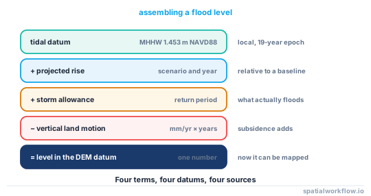
Get every component into one vertical datum before adding anything:
FLOOD_LEVEL_M = (
    mhhw_in_navd88          # the tidal surface, converted through the gauge datums
    + projected_rise_m      # the scenario, relative to a stated baseline period
    + storm_allowance_m     # the return-period surge, if you are mapping a flood
    - vertical_land_motion  # subsidence adds, uplift subtracts
)
Every term needs a datum, a baseline period and a source. At Boston, MHHW is 1.453 m above NAVD88, so a scenario of +0.5 m by 2100 maps to a still-water level of 1.953 m NAVD88 before any storm allowance.
Step-by-step solution
1. Distinguish the four quantities
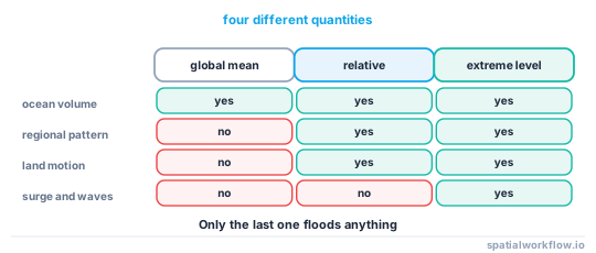
- Global mean sea level — the ocean-volume average from satellite altimetry since 1993 and from tide gauges before that. A single global number.
- Regional sea level change — the same quantity with ocean dynamics, gravity and ice-mass fingerprints included. Varies by a factor of two or more between regions.
- Relative sea level — what a tide gauge measures: the sea relative to the land it is bolted to, so it includes vertical land motion.
- Extreme water level — the still water plus the surge and wave setup for a given return period. This is what floods anything.
A projection published as "global mean" is not the number to add at a specific place.
2. Get the vertical land motion right
Land subsidence adds directly to relative sea level rise and can exceed the climatic signal. Subsiding deltas and formerly glaciated coasts move in opposite directions, and GNSS or InSAR rates are the source.
3. Read the baseline period of the projection
A projection of "+0.5 m by 2100" is relative to a baseline — often 1995–2014 or 2000. Adding it to a present-day tidal datum from the 1983–2001 epoch double-counts the rise that has already happened between the two.
4. Choose a scenario and name it
Projections come as scenarios with likely ranges and low-confidence high-end branches. A map showing one number without naming the scenario, the percentile and the year is not interpretable.
5. Convert the tidal surface into the terrain model's datum
This is the step that gets skipped. Terrain models are in a national orthometric datum; tidal datums are local and published relative to station datum. Convert through the gauge's published offsets.
6. Add a storm allowance if you are mapping flooding
Still-water sea level rise alone floods almost nothing new. The damaging events are surges on top of a high tide, and the return-period level is what coastal flood maps are actually drawn at.
7. Publish the uncertainty
Every term has one: the projection range, the land motion rate, the DTM's vertical error, and the datum conversion. A single contour implies a precision none of them supports.
Code examples
Example 1 — assemble the flood level with every term named
import dataclasses, json

@dataclasses.dataclass
class FloodLevel:
    tidal_datum: str              # e.g. "MHHW"
    tidal_datum_m_navd88: float   # from the gauge's published offsets
    scenario: str                 # e.g. "intermediate, 50th percentile"
    baseline_period: str          # e.g. "2000"
    projected_rise_m: float
    year: int
    storm_return_period_years: int | None
    storm_allowance_m: float
    vertical_land_motion_mm_yr: float
    reference_year: int = 2026

    def level_m_navd88(self):
        vlm = (self.vertical_land_motion_mm_yr / 1000) * (self.year - self.reference_year)
        return (self.tidal_datum_m_navd88 + self.projected_rise_m
                + self.storm_allowance_m - vlm)

f = FloodLevel(tidal_datum="MHHW", tidal_datum_m_navd88=1.453,
               scenario="intermediate, 50th percentile", baseline_period="2000",
               projected_rise_m=0.50, year=2100,
               storm_return_period_years=100, storm_allowance_m=1.20,
               vertical_land_motion_mm_yr=-1.5)
print(json.dumps(dataclasses.asdict(f) | {"level_m_navd88": round(f.level_m_navd88(), 3)},
                 indent=2))
A dataclass rather than a float, so the number cannot travel without its assumptions. Note that the subsidence term uses a negative rate — land going down raises relative sea level.
Example 2 — the trend from a real gauge record
import urllib.request, json, numpy as np, pandas as pd

def monthly_means(station, begin_year, end_year):
    frames = []
    for y in range(begin_year, end_year + 1):
        url = (f"https://api.tidesandcurrents.noaa.gov/api/prod/datagetter"
               f"?product=monthly_mean&application=spatialworkflow-docs"
               f"&begin_date={y}0101&end_date={y}1231&datum=MSL&station={station}"
               f"&time_zone=gmt&units=metric&format=json")
        with urllib.request.urlopen(url, timeout=120) as r:
            raw = json.loads(r.read())
        if "data" in raw:
            frames.append(pd.DataFrame(raw["data"]))
    df = pd.concat(frames, ignore_index=True)
    df["t"] = pd.to_datetime(df["year"] + "-" + df["month"].str.zfill(2) + "-01")
    df["msl"] = pd.to_numeric(df["MSL"], errors="coerce")
    return df.dropna(subset=["msl"])

df = monthly_means("8443970", 1990, 2025)
x = (df["t"] - df["t"].min()).dt.days / 365.25
slope, _ = np.polyfit(x, df["msl"], 1)
print(f"{len(df)} monthly means, trend {slope * 1000:.2f} mm/yr")
A gauge trend is relative sea level: it includes whatever the land is doing. Comparing it with a global mean number without separating vertical land motion is the classic mistake.
Example 3 — a scenario sweep rather than a single line
import numpy as np, rasterio
from rasterio.features import shapes
from shapely.geometry import shape

SCENARIOS = {"low": 0.30, "intermediate": 0.50, "high": 1.00, "extreme": 2.00}

with rasterio.open("dtm_navd88.tif") as src:
    dtm = src.read(1, masked=True)
    transform, crs = src.transform, src.crs

base = 1.453           # MHHW in NAVD88
for name, rise in SCENARIOS.items():
    level = base + rise
    below = (dtm <= level).filled(False)
    area_km2 = below.sum() * abs(transform.a * transform.e) / 1e6
    print(f"{name:13} +{rise:.2f} m → level {level:.3f} m NAVD88, "
          f"{area_km2:,.1f} km² below")
Publish the sweep, not one scenario. The difference between the low and high lines is the honest message, and a single contour hides it.
Explanation
Why global and local numbers differ so much
Sea level is not flat. Ocean currents, thermal expansion patterns, and the gravitational fingerprint of melting ice sheets — meltwater from Greenland raises sea level less nearby and more in the far field — all mean regional change departs substantially from the global mean. Add vertical land motion and the relative change at a gauge can be several times the global figure or, on rebounding coasts, negative.
Why still-water rise alone maps almost nothing
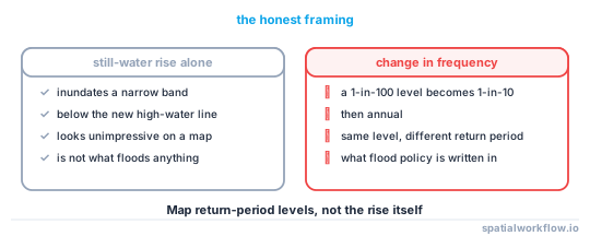
Half a metre of still-water rise inundates only land below half a metre above the present high-water line, which is a narrow band. What changes is the frequency of extremes: an event that used to be a 1-in-100-year level becomes a 1-in-10 or annual one. That is the honest way to present the result, and it is why a coastal flood map is drawn at a return-period level rather than at the rise itself.
Why the baseline period is a real source of double counting
Both the tidal datum and the projection are anchored to a period. A datum from the 1983–2001 epoch already reflects the sea level of the 1990s; a projection relative to 2000 counts from roughly the same point, so adding them is approximately right. A projection relative to 1900 added to a modern datum counts the twentieth century twice.
Why the terrain model's error belongs in the total
A LiDAR DTM has a vertical RMSE of 0.1–0.3 m in open terrain and worse in vegetation and on soft ground. Against a scenario of 0.5 m that is a large fraction of the signal, which is why inundation extents should be presented as a band rather than a line.
Edge cases or notes
- Relative and absolute differ by the land motion. Say which you are using.
- Tide gauge records need datum continuity. Gauges are moved and re-levelled.
- Altimetry starts in 1993. Earlier global series are gauge reconstructions.
- Scenario percentiles matter. A 50th and a 95th differ by a factor of two or more.
- Wave setup and runup are on top of surge, and are not in a still-water level.
- Groundwater and drainage flood inland before the sea reaches there.
- Defences are not in a DTM. A bathtub map floods behind seawalls.
- State every datum. The commonest error is arithmetic between different zeros.
Internal links
- Tidal datums explained: which shoreline is the shoreline — converting the tidal surface
- How to map coastal inundation from a DEM in Python — turning a level into an extent
- An inundation map floods inland areas that cannot flood — what a bathtub fill gets wrong
- How to fetch and align tide gauge data in Python — the observations behind a trend
- Vertical datums explained — the arithmetic between zeros
- Bathymetry explained: depths, datums and grids — the offshore side of the same question
- Digital elevation models explained — the terrain model's own error
- Height above nearest drainage explained — a better proxy than an elevation threshold
FAQ
What is the difference between global and relative sea level rise?
Global mean is the ocean-volume average. Relative is what a gauge measures at a place, including regional ocean dynamics and vertical land motion, and it can be several times the global figure.
Can I add a projected rise to my DEM?
Only after converting both to the same vertical datum, and only after adding the tidal surface. A rise added to a bare DEM zero is a map of nothing in particular.
Why does still-water rise flood so little?
Because it only inundates the narrow band below the new high-water line. The real effect is that extreme levels become far more frequent, which is why flood maps use return-period levels.
Which scenario should I map?
Several, and name each one with its percentile and year. A single contour implies a certainty that no projection supports.
Does land subsidence matter?
Often more than the climatic signal. In subsiding deltas it dominates relative sea level rise; on rebounding coasts it partly cancels it.
How accurate is the resulting extent?
No better than the DTM, which is typically 0.1–0.3 m RMSE — a large fraction of a half-metre scenario. Present a band, not a line.