Tide times are off by hours after a join

Problem statement

The tide level attached to each event is wrong, and wrong by an amount that looks like a whole tide. High water in the joined table sits near mid-tide. The residual between observation and prediction is most of a metre rather than a few centimetres.

This page reproduces it with real data from NOAA's gauge at The Battery, New York (station 8518750), for 1–20 March 2025 — a window that contains the switch to daylight saving time on 9 March. The "events" are the 77 high and low waters from NOAA's own tide table for the station, requested in local time the way a tide table is printed; the gauge readings are six-minute observations requested in GMT. Joining the two naively:

naive = pd.merge_asof(events.assign(time=pd.to_datetime(events["t"])).sort_values("time"),
                      gauge.assign(time=pd.to_datetime(gauge["t"]))[["time", "v"]]
                           .rename(columns={"v": "observed"}),
                      on="time", direction="nearest")
highs = naive["type"] == "H"
print(f"high waters: predicted {naive.loc[highs, 'v'].mean():.2f} m, "
      f"observed at the joined time {naive.loc[highs, 'observed'].mean():.2f} m")

high waters: predicted 1.38 m, observed at the joined time 0.41 m

Every high water joined to a gauge reading four or five hours too early — the local clock read as UTC — and the "observed" level at high water is less than a third of the predicted one.

There are five causes, and each has a signature you can read from the joined series against the raw one: a naive local timestamp read as UTC, a local-time request joined to UTC data, daylight saving, a datum mismatch that looks like a time error, and a nearest-time join that reached across a gap.

Quick answer

Make every timestamp timezone-aware at the boundary, and join with a tolerance:

gauge_utc = gauge.assign(time=pd.to_datetime(gauge["t"]).dt.tz_localize("UTC"))  # asked for GMT
events_utc = events.assign(time=pd.to_datetime(events["t"])
                           .dt.tz_localize("America/New_York")                     # the table is local
                           .dt.tz_convert("UTC"))

joined = pd.merge_asof(events_utc.sort_values("time"),
                       gauge_utc[["time", "v"]].rename(columns={"v": "observed"}).sort_values("time"),
                       on="time", direction="nearest", tolerance=pd.Timedelta("15min"))
highs = joined["type"] == "H"
print(f"{joined['observed'].isna().sum()} of {len(joined)} events had no reading within 15 min")
print(f"high waters: predicted {joined.loc[highs, 'v'].mean():.2f} m, observed {joined.loc[highs, 'observed'].mean():.2f} m")

0 of 77 events had no reading within 15 min
high waters: predicted 1.38 m, observed 1.51 m

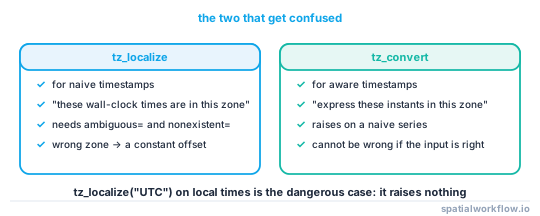
tz_localize attaches a zone to a naive timestamp; tz_convert changes the zone of an aware one. Localising the tide table to New York before converting to UTC is what moved every event the right four or five hours — five before 9 March, four after — and the remaining gap between predicted and observed is the weather, not the clock.

Read the offset, request GMT, localise naive times

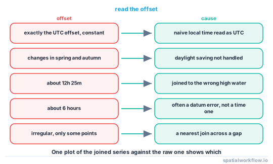
1. Read the offset, because it names the cause

At The Battery the first two are the same mistake measured on either side of 9 March: five hours in EST, four in EDT.

2. Request GMT from the API

time_zone=gmt on the NOAA datagetter returns UTC timestamps, which removes daylight saving from the problem entirely. lst_ldt returns local standard or daylight time depending on the date — and around the change it does something more awkward:

local = noaa("water_level", "lst_ldt")
t = pd.to_datetime(local["t"])
print(len(gauge), "rows in GMT,", len(local), "rows in lst_ldt")
print(local[(t >= "2025-03-09 01:54") & (t <= "2025-03-09 03:00")][["t", "v"]].to_string(index=False))

4800 rows in GMT, 4800 rows in lst_ldt
               t     v
2025-03-09 01:54 0.785
2025-03-09 02:00   NaN
2025-03-09 02:06   NaN
2025-03-09 02:12   NaN
2025-03-09 02:18   NaN
2025-03-09 02:24   NaN
2025-03-09 02:30   NaN
2025-03-09 02:36   NaN
2025-03-09 02:42   NaN
2025-03-09 02:48   NaN
2025-03-09 02:54   NaN
2025-03-09 03:00 0.817

The local-time response has ten rows stamped 02:00 to 02:54 on 9 March, an hour that did not exist in New York, each with an empty value. The GMT response for the same window has no hole. A join on the local series quietly gains ten blank readings at the one hour of the year when the clock is least trustworthy.

3. Localise, do not convert, a naive timestamp

stamps = pd.to_datetime(local["t"])
aware = stamps.dt.tz_localize("America/New_York", ambiguous="NaT", nonexistent="NaT")
print("nonexistent local times:", aware.isna().sum())
print("offsets seen:", sorted(aware.dropna().map(lambda ts: ts.strftime("%z")).unique()))
try:
    stamps.dt.tz_localize("America/New_York")
except Exception as exc:
    print("without nonexistent=:", type(exc).__name__, str(exc)[:50])

nonexistent local times: 10
offsets seen: ['-0400', '-0500']
without nonexistent=: ValueError 2025-03-09 02:00:00 is a nonexistent time due to d

ambiguous="NaT" and nonexistent="NaT" make the two daylight-saving edge cases explicit rather than guessed: an hour that occurs twice in autumn and one that does not exist in spring. Without them, pandas refuses the whole series — which is better than guessing, and worse than knowing exactly which ten rows are the problem.

4. Check whether the error is actually a datum error

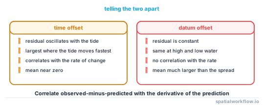
A constant offset in level rather than time can look like a time error on a plot, because a tide curve shifted vertically resembles one shifted horizontally near the turning points. NOAA publishes the same predictions against several datums; asking for mean sea level (MSL) instead of mean lower low water (MLLW) is the classic slip:

msl = noaa("predictions", "gmt", datum="MSL")
offset = (predicted["v"].values - msl["v"].values)
print(f"MLLW minus MSL predictions: mean {offset.mean():.3f} m, spread {offset.std():.4f} m")

MLLW minus MSL predictions: mean 0.783 m, spread 0.0001 m

The two differ by 0.783 m at every one of the 4,800 six-minute steps. Compared with observations, a level offset appears as a constant residual; a time offset as a residual that oscillates with the tide. Example 3 separates them.

5. Join with a tolerance

merge_asof with direction="nearest" always finds a match. On six-minute data every event is within three minutes of a reading; on NOAA's hourly heights for the same gauge it is not:

hourly = noaa("hourly_height", "gmt")
hourly_utc = hourly.assign(time=pd.to_datetime(hourly["t"]).dt.tz_localize("UTC"))
for tol in (None, pd.Timedelta("15min")):
    j = pd.merge_asof(events_utc.sort_values("time"),
                      hourly_utc[["time", "v"]].rename(columns={"v": "observed"}),
                      on="time", direction="nearest", tolerance=tol)
    print(f"tolerance {str(tol):16} unmatched {j['observed'].isna().sum()} of {len(j)}")

tolerance None             unmatched 0 of 77
tolerance 0 days 00:15:00  unmatched 34 of 77

Without a tolerance every event is matched, some to a reading up to half an hour away, and nothing says so. With one, the events too far from a reading become NaN you can count — 34 of the 77 here, which is the next step's point.

6. Check the sampling interval

Six-minute data joined at a 15-minute tolerance is fine. Hourly data joined at the same tolerance left 34 of 77 events unmatched, and high_low data is irregular by construction — it is itself a list of events, not a series to interpolate.

7. Validate on a known high water

Pick the predicted high waters and check that the observed series peaks within a few minutes of each:

obs = gauge_utc.set_index("time")["v"]
lags = []
for when in events_utc.loc[events_utc["type"] == "H", "time"]:
    window = obs[when - pd.Timedelta("1h"): when + pd.Timedelta("1h")]
    lags.append((window.idxmax() - when).total_seconds() / 60)
lags = pd.Series(lags)
print(f"{len(lags)} high waters: observed peak minus predicted, median {lags.median():+.0f} min, "
      f"middle half {lags.quantile(0.25):+.0f} to {lags.quantile(0.75):+.0f} min")

38 high waters: observed peak minus predicted, median +12 min, middle half +1 to +21 min

A median within a quarter of an hour, and a spread of a few tens of minutes that is the weather and a flat tide top, is what a correct join looks like: the observed peaks came a median 12 minutes after the predicted ones. A median of −240 or −300 is the time-zone mistake; ±745 is the wrong tide.

Measuring the offset instead of guessing

The data used on this page

Six-minute water levels, six-minute predictions and high/low predictions for The Battery, NY (8518750) from the NOAA CO-OPS data API, 1–20 March 2025, metric, cached on first run. NOAA data are public domain.

import json
from pathlib import Path

import numpy as np
import pandas as pd
import requests

API = "https://api.tidesandcurrents.noaa.gov/api/prod/datagetter"
Path("data").mkdir(exist_ok=True)


def noaa(product, time_zone, datum="MLLW", **extra):
    """One CO-OPS request for The Battery, 1-20 March 2025, cached as JSON."""
    cache = Path(f"data/{product}_{time_zone}_{datum}_{'_'.join(extra.values())}.json")
    if not cache.exists():
        params = {"station": "8518750", "product": product, "datum": datum, "time_zone": time_zone,
                  "units": "metric", "format": "json", "begin_date": "20250301", "end_date": "20250320",
                  "application": "spatialworkflow.io", **extra}
        cache.write_text(requests.get(API, params=params, timeout=120).text)
    body = json.loads(cache.read_text())
    rows = pd.DataFrame(body["predictions"] if "predictions" in body else body["data"])
    rows["v"] = pd.to_numeric(rows["v"], errors="coerce")
    return rows


gauge = noaa("water_level", "gmt")                           # observed, UTC
predicted = noaa("predictions", "gmt")                        # six-minute predictions, UTC
events = noaa("predictions", "lst_ldt", interval="hilo")      # the local tide table
print(f"{len(gauge):,} readings, {len(predicted):,} predictions, {len(events)} high/low waters "
      f"({(events['type'] == 'H').sum()} high)")
print(events.head(3).to_string(index=False))

4,800 readings, 4,800 predictions, 77 high/low waters (38 high)
               t      v type
2025-03-01 03:01 -0.280    L
2025-03-01 08:52  1.624    H
2025-03-01 15:23 -0.330    L

Example 1 — measure the offset rather than guessing it

def time_offset(observed, predicted, max_lag_min=360, step_min=6):
    """Cross-correlate two regular six-minute series to find the lag that aligns them."""
    o = observed.astype(float)
    p = predicted.astype(float).reindex(o.index).interpolate()
    best, best_r = 0, -np.inf
    for lag in range(-max_lag_min, max_lag_min + 1, step_min):
        shifted = p.shift(lag // step_min)
        ok = o.notna() & shifted.notna()
        if ok.sum() < 100:
            continue
        r = float(np.corrcoef(o[ok], shifted[ok])[0, 1])
        if r > best_r:
            best, best_r = lag, r
    return {"lag_minutes": best, "correlation": round(best_r, 4)}

obs = pd.Series(gauge["v"].values, index=pd.to_datetime(gauge["t"]))
pred = pd.Series(predicted["v"].values, index=pd.to_datetime(predicted["t"]))
local_pred = noaa("predictions", "lst_ldt")
pred_local_as_utc = pd.Series(local_pred["v"].values, index=pd.to_datetime(local_pred["t"]))
print("GMT predictions:              ", time_offset(obs, pred))
print("local predictions read as UTC:", time_offset(obs, pred_local_as_utc))

GMT predictions:               {'lag_minutes': 0, 'correlation': 0.9472}
local predictions read as UTC: {'lag_minutes': 270, 'correlation': 0.9156}

A lag of 0 with a high correlation means the alignment is right; 0.947 rather than 1 is the weather, which no prediction contains. The local predictions read as UTC give 270 minutes — neither the five hours of EST nor the four of EDT but a compromise between them, because one lag has to fit a window that spans the clock change. A lag of whole hours is a time-zone offset; a lag near 745 minutes is a whole tidal cycle, outside this search on purpose.

Example 2 — a timestamp parser that refuses to guess

def to_utc(series, source_tz=None, assume_utc=False):
    s = pd.to_datetime(series, errors="coerce")
    if s.dt.tz is not None:
        return s.dt.tz_convert("UTC")
    if assume_utc:
        return s.dt.tz_localize("UTC")
    if source_tz is None:
        raise ValueError("naive timestamps and no source_tz: state the zone, or pass assume_utc=True")
    return s.dt.tz_localize(source_tz, ambiguous="NaT", nonexistent="NaT").dt.tz_convert("UTC")

try:
    to_utc(events["t"])
except ValueError as exc:
    print("ValueError:", exc)
converted = to_utc(events["t"], source_tz="America/New_York")
print(f"{converted.isna().sum()} event times were ambiguous or nonexistent; first event {converted.iloc[0]}")
local_readings = to_utc(noaa("water_level", "lst_ldt")["t"], source_tz="America/New_York")
print(f"{local_readings.isna().sum()} of the local gauge's timestamps were nonexistent")

ValueError: naive timestamps and no source_tz: state the zone, or pass assume_utc=True
0 event times were ambiguous or nonexistent; first event 2025-03-01 08:01:00+00:00
10 of the local gauge's timestamps were nonexistent

Raising on a naive timestamp with no stated zone is the point. Every silent default here is a four- or five-hour error somewhere downstream.

Example 3 — separate a time error from a datum error

def residual_signature(observed, predicted):
    both = pd.concat([observed, predicted], axis=1, keys=["obs", "pred"]).dropna()
    r = both["obs"] - both["pred"]
    rate = both["pred"].diff()                   # a time offset correlates with the rate of change
    ok = r.notna() & rate.notna()
    corr = float(np.corrcoef(r[ok], rate[ok])[0, 1])
    return {"mean_residual_m": round(float(r.mean()), 3),
            "sd_residual_m": round(float(r.std()), 3),
            "corr_with_rate": round(corr, 3),
            "likely": "datum offset" if abs(r.mean()) > 2 * r.std()
                      else "time offset" if abs(corr) > 0.5 else "meteorological"}

msl_pred = pd.Series(noaa("predictions", "gmt", datum="MSL")["v"].values, index=pred.index)
print("correct:          ", residual_signature(obs, pred))
print("MSL datum:        ", residual_signature(obs, msl_pred))
print("predictions +1 h: ", residual_signature(obs, pred.shift(10)))

correct:           {'mean_residual_m': 0.145, 'sd_residual_m': 0.17, 'corr_with_rate': -0.008, 'likely': 'meteorological'}
MSL datum:         {'mean_residual_m': 0.928, 'sd_residual_m': 0.17, 'corr_with_rate': -0.008, 'likely': 'datum offset'}
predictions +1 h:  {'mean_residual_m': 0.143, 'sd_residual_m': 0.303, 'corr_with_rate': 0.789, 'likely': 'time offset'}

The correlation with the rate of change is the discriminator: a series shifted in time has its largest residuals where the tide is moving fastest, while a datum error has the same residual everywhere. The correct pair is left with a mean residual of 0.145 m and a spread of 0.17 m that follows neither — that is surge and wind, the part of the water level no tide table predicts. The MSL predictions have exactly the same spread and correlation, with the mean moved by the 0.783 m between the datums.

Localise versus convert

Why tz_localize and tz_convert are so easy to confuse

tz_localize says "these wall-clock times are in this zone"; tz_convert says "express these known instants in this zone". Applied to a naive series, tz_convert raises, which is helpful. Applied to an aware series, tz_localize raises too. The dangerous case is tz_localize("UTC") on a series that was recorded in local time — it produces an aware series that is wrong by the offset and raises nothing, which is exactly the join in the problem statement.

Why GMT removes most of the problem

Requesting local time from an API means the returned timestamps change their offset twice a year, and the transition hours are ambiguous or nonexistent — NOAA even returns rows for the hour that does not exist. UTC has neither property. Converting to local time for display at the very end is easy; parsing local time at the input boundary is not.

Why a level error can look like a time error

Near high and low water the tide curve is flat, so a vertical shift and a horizontal shift produce similar-looking displacement there. On the steep part of the curve they differ: a time shift produces a residual proportional to the rate of change, while a datum offset produces a constant one. Correlating the residual with the derivative separates them in one line.

Why a nearest join needs a tolerance

merge_asof with direction="nearest" always finds a match. If the gauge has a gap — ice, maintenance, a failed sensor — or is simply sampled hourly, an event is matched to an observation far away, which on a semidiurnal tide can be a quite different state. A tolerance makes the distance visible as a NaN, and counting them is the check.

Ambiguous times and standard-time gauges

• ambiguous and nonexistent must be set for any local-time localisation.
• Some gauges report in local standard time year-round. Read the metadata.
• high_low products are irregular and must not be resampled.
• Leap seconds are not in pandas. They are below the noise here.
• Survey timestamps may be the file's mtime. Check what the field means.
• Satellite acquisition times are UTC. Join to UTC gauge data directly.
• A whole-cycle error is 12h 25m, not 12h — semidiurnal, not solar.
• Plot the joined series once. Every one of these is visible.

Internal links

• How to fetch and align tide gauge data in Python — the fetch and join done properly
• Tidal datums explained: which shoreline is the shoreline — the datum half of the confusion
• Spatial data has timezone errors in the time column — the same problem in general
• How to standardise dates in spatial data with Python — parsing at the boundary
• How to measure shoreline change between two dates — where the tide state is needed
• How to resample a time series in xarray — resampling without crossing gaps
• cftime and datetime errors in xarray — calendars in gridded data
• Sea level rise data explained — the residual as the interesting series

FAQ

Why is my joined tide level wrong by a constant amount of time?

Almost always a naive local timestamp localised as UTC. The error equals the UTC offset and is constant outside daylight-saving transitions.

What is the difference between tz_localize and tz_convert?

tz_localize attaches a zone to naive times; tz_convert re-expresses aware times in another zone. Using the first on local times labelled as UTC is the classic bug.

Why does the offset change twice a year?

Daylight saving. Request GMT from the API and convert to local only for display.

How do I tell a time error from a datum error?

Correlate the observed-minus-predicted residual with the rate of change of the tide. A time shift correlates; a datum offset is constant.

Why did some events get a tide level from six hours away?

Because merge_asof with direction="nearest" has no tolerance by default. Set one, and count the NaNs.

How do I verify the join?

Pick a date, look up the predicted high water, and check the joined series peaks within a few minutes of it.