
How to load and plot a bathymetry grid in Python
Problem statement
A global bathymetry grid is large — ETOPO 2022 at one arc-minute is 10,800 × 21,600 cells and 933 MB in memory as float32 — so the first thing to get right is not loading all of it. The second is the sign convention, because a plot of depth where the data is elevation is upside down in colour and nobody notices.
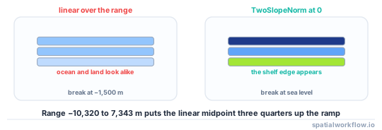
The third is the colour ramp. With 37% of the planet in a single 2,000 m depth band and a total range of 17,663 m, a linear ramp over the full range shows a uniform blue ocean and a uniform brown land.
This guide loads a subset efficiently, establishes the convention, and produces a plot that shows the structure that is actually there.
Quick answer
import xarray as xr, numpy as np
import matplotlib.pyplot as plt
import matplotlib.colors as mcolors

ds = xr.open_dataset("etopo_2022_60s.nc")          # lazy: nothing is read yet
z = ds["z"].sel(lat=slice(51.0, 56.0), lon=slice(1.0, 9.0)).load()
print(z.attrs["positive"], z.shape, float(z.min()), float(z.max()))

norm = mcolors.TwoSlopeNorm(vmin=float(z.min()), vcenter=0, vmax=float(z.max()))
fig, ax = plt.subplots(figsize=(8, 6))
im = z.plot.imshow(ax=ax, cmap="topo", norm=norm, add_colorbar=False)
fig.colorbar(im, ax=ax, label="elevation (m, EGM2008)")
TwoSlopeNorm with vcenter=0 is the single most useful line: it puts the colour break at sea level rather than at the midpoint of the range, which is what makes a bathymetry map readable.
Step-by-step solution
1. Open lazily and subset before loading
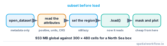
xr.open_dataset reads metadata only. Selecting a region and calling .load() reads just that block — for the North Sea box above, 300 × 480 cells rather than 233 million.
2. Read the convention from the attributes
print(dict(ds["z"].attrs)){'long_name': 'z', 'units': 'meters', 'positive': 'up', 'standard_name': 'height',
'vert_crs_name': 'EGM2008', 'vert_crs_epsg': 'EPSG:3855'}
positive: up means elevation, so the sea is negative. If the attribute is missing, probe a point you know is deep ocean.
3. Mask land and sea separately
Most bathymetric work wants one or the other. z.where(z < 0) gives the sea with land as NaN, which is also what you want before computing any ocean statistic.
4. Choose the colour scheme deliberately
Three that work:
- Two-slope norm centred on zero with a topo-bathy colormap — the general-purpose answer.
- Sea only, with a sequential ramp over the actual depth range in that region — best for a shelf sea where the global range is irrelevant.
- Quantile classes — best when the distribution is strongly skewed and you want equal numbers of cells per class.
5. Add contours for the structure a ramp cannot show
Depth contours at 20, 50, 100, 200 and 1,000 m communicate the shelf, the slope and the abyss far better than colour alone.
6. Do not plot 233 million cells
Decimating by a factor of eight before a global plot reduces the array by 64 times and changes nothing you can see at screen resolution. For a figure, decimate; for analysis, do not.
7. Check the longitude convention
Some grids run 0–360 rather than −180 to 180. Subsetting across the antimeridian on such a grid needs a roll rather than a slice.
Code examples
Example 1 — load a region and describe it
import xarray as xr, numpy as np

def load_region(path, lat_slice, lon_slice, var="z"):
    ds = xr.open_dataset(path)
    a = ds[var].sel(lat=slice(*lat_slice), lon=slice(*lon_slice)).load()
    report = {
        "shape": a.shape,
        "attrs": dict(a.attrs),
        "range_m": (float(a.min()), float(a.max())),
        "sea_fraction": float((a < 0).mean()),
        "mean_depth_m": float(-a.where(a < 0).mean()),
    }
    return a, report

z, r = load_region("etopo_2022_60s.nc", (51.0, 56.0), (1.0, 9.0))
print(r["shape"], r["range_m"], f"{r['sea_fraction']:.1%}", f"{r['mean_depth_m']:.1f} m")
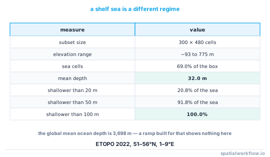
(300, 480) (-93.0, 775.0) 69.0% 32.0 m
A shelf sea: nothing below 100 m, a mean depth of 32 m, and a colour ramp built for the global range would render all of it one shade.
Example 2 — a readable plot with contours
import matplotlib.pyplot as plt
import matplotlib.colors as mcolors
import numpy as np

def plot_bathymetry(z, contours=(-200, -100, -50, -20, -10), figsize=(9, 7)):
    fig, ax = plt.subplots(figsize=figsize)
    vmin, vmax = float(z.min()), float(z.max())
    norm = mcolors.TwoSlopeNorm(vmin=vmin, vcenter=0, vmax=max(vmax, 1))

    im = ax.pcolormesh(z["lon"], z["lat"], z.values, cmap="terrain", norm=norm,
                       shading="auto")
    cs = ax.contour(z["lon"], z["lat"], z.values, levels=sorted(contours),
                    colors="#1a3a6b", linewidths=0.6)
    ax.clabel(cs, fmt=lambda v: f"{abs(v):.0f} m", fontsize=7)

    ax.set_aspect(1 / np.cos(np.deg2rad(float(z["lat"].mean()))))
    fig.colorbar(im, ax=ax, label="elevation (m)")
    return fig, ax
The aspect ratio line matters: plotting a geographic grid with an aspect of 1 stretches everything east–west by 1/cos(latitude), which at 54°N is a 70% distortion.
Example 3 — sea-only, with a ramp fitted to the region
import numpy as np, matplotlib.pyplot as plt

sea = z.where(z < 0)
d = -sea.values
d = d[np.isfinite(d)]

fig, ax = plt.subplots(figsize=(9, 7))
im = ax.pcolormesh(z["lon"], z["lat"], -sea.values, cmap="Blues",
                   vmin=0, vmax=np.percentile(d, 99), shading="auto")
ax.set_aspect(1 / np.cos(np.deg2rad(float(z["lat"].mean()))))
fig.colorbar(im, ax=ax, label="depth (m)")
print(f"ramp fitted to 0–{np.percentile(d, 99):.0f} m "
      f"(the deepest 1% of cells clip)")
Clipping at the 99th percentile rather than the maximum stops a single deep hole from compressing the rest of the ramp — the same reason a satellite image is stretched to percentiles rather than to its extremes.
Explanation
Why lazy loading matters so much here
The full ETOPO array is 933 MB as float32 and considerably more once NumPy makes a copy. Most questions concern a region, and sel on a lazily opened dataset reads only the blocks that intersect the selection. The habit is worth keeping even for small files, because it makes the same code work when the file becomes a Zarr store on object storage.
Why positive: up is worth trusting and checking
It is the CF convention's explicit statement of the sign, and it is the only authoritative one. It can still be wrong if somebody negated the array without updating the attribute, which is why probing a known deep point costs one line and settles the question.
Why the colour break belongs at zero
A linear ramp maps the midpoint of the data range to the middle colour. With a range of −10,320 to 7,343 m, that midpoint is about −1,500 m, so sea level falls three quarters of the way up the ramp and the land-sea boundary is invisible. TwoSlopeNorm fixes the break at zero and scales each side independently.
Why the plot aspect ratio is not cosmetic
A geographic grid plotted with equal axis scaling is a plate carrée projection, which stretches east–west by 1/cos(latitude). At 54°N that is a factor of 1.70, which distorts every shape and makes a circular feature look like an ellipse. Setting the aspect to 1/cos(mean latitude) is a one-line approximation that removes most of it.
Edge cases or notes
- Slices must match the coordinate order. If
latis descending,slice(56, 51). - Longitude 0–360 grids need a roll to subset across the antimeridian.
.load()is the moment memory is used. Check the shape first.- NaN versus a fill value. −9999 plots as a trench if it is not masked.
- Decimate for figures only. Statistics on a decimated grid need re-weighting.
pcolormeshwants cell edges;shading="auto"handles centres.- Colormaps named
topovary between libraries;terrainis in matplotlib. - Add the vertical datum to the colourbar label. It is part of the number.
Internal links
- Bathymetry explained: depths, datums and grids — the conventions behind the numbers
- How to generate depth contours from bathymetry — the contours in this plot, properly
- Bathymetry depths are positive in one file and negative in another — when two grids disagree
- How to open NetCDF files with xarray in Python — the loading pattern in general
- How to select time and location in xarray — subsetting before loading
- Lazy loading in xarray explained — why
selbeforeloadmatters - How to design a colour ramp in Python — choosing the classes
- How to subset an ocean model NetCDF by depth and time — the four-dimensional version
FAQ
How do I load a global bathymetry grid without running out of memory?
Open it lazily with xr.open_dataset, select the region with sel, and only then call .load(). The full ETOPO array is 933 MB; a North Sea box is 300 × 480 cells.
How do I know whether the values are depths or elevations?
Read the CF positive attribute. ETOPO 2022 declares positive: up, so the sea is negative. If it is missing, probe a point you know is deep ocean.
Why does my bathymetry map look like one flat colour?
Because a linear ramp over the full range puts the colour break at about −1,500 m. Use TwoSlopeNorm with vcenter=0.
Why is my map stretched sideways?
A geographic grid plotted with equal axis scaling stretches east–west by 1/cos(latitude) — a factor of 1.70 at 54°N. Set the aspect to 1/cos(mean latitude).
Should I decimate the grid?
For figures, yes — a factor of eight changes nothing visible and reduces the array 64-fold. For statistics, no.
What contour intervals should I use?
Choose them for the region: 10, 20, 50, 100 and 200 m on a shelf sea; 1,000 m intervals offshore. A single global interval shows nothing in either place.