
How to generate depth contours from bathymetry
Problem statement
Depth contours from a grid are a contour call, and the two decisions around it — the interval and the smoothing — decide whether the result is a chart or a mess.
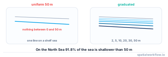
The interval is not a style choice. Bathymetry is strongly bimodal: on the North Sea shelf, 91.8% of the sea area is shallower than 50 m and nothing is deeper than 100 m, while offshore the same region's neighbours drop through four kilometres. A single interval that works in one shows nothing in the other.
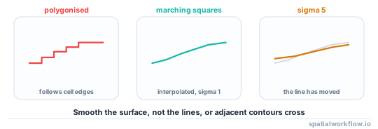
The smoothing is the other half. A contour traced directly from a grid follows cell boundaries, so it comes out as a staircase at the grid resolution, and every contour crosses itself wherever the surface is noisy.
Quick answer
Choose the levels from the distribution, smooth the surface rather than the lines:
import numpy as np, xarray as xr, geopandas as gpd
from scipy import ndimage
from skimage import measure
from shapely.geometry import LineString

def depth_contours(z, transform, levels, smooth_sigma=1.0):
    """z: 2D array of elevation (negative at sea); levels: negative values."""
    surface = ndimage.gaussian_filter(np.nan_to_num(z, nan=np.nanmax(z)), smooth_sigma)
    out = []
    for level in levels:
        for c in measure.find_contours(surface, level):
            xs, ys = transform * (c[:, 1], c[:, 0])
            if len(xs) >= 2:
                out.append({"depth_m": abs(level), "geometry": LineString(zip(xs, ys))})
    return gpd.GeoDataFrame(out)
find_contours uses marching squares with linear interpolation between cells, so the line runs through cells rather than around them — which removes the staircase without any line simplification.
Step-by-step solution
1. Look at the depth distribution first
d = -z[z < 0]
print(np.percentile(d, [5, 25, 50, 75, 95]).round(0))
On the North Sea box the sea is 69.0% of the area with a mean depth of 32.0 m and nothing below 100 m; on a global grid the median ocean depth is 3,909 m. The contour set follows from that, not from a convention.
2. Use a non-uniform interval
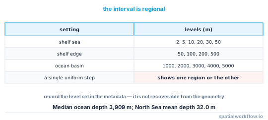
The standard chart approach is fine intervals in shallow water and coarse ones offshore: 2, 5, 10, 20, 30, 50, 100, 200, 500, 1000, 2000, 4000 m. That is a set of levels, not a step.
3. Smooth the surface, not the contours
Gaussian smoothing of the grid before contouring gives lines that are smooth and consistent with each other. Simplifying the lines afterwards gives lines that cross, because neighbouring contours are simplified independently.
4. Choose the smoothing from the data, not from the look
A sigma of one cell removes single-cell noise. Larger values start moving the contours: a sigma of three cells on a 1.85 km grid displaces a contour by up to several kilometres on a steep slope. Check the displacement against the unsmoothed version.
5. Handle the land-sea boundary
The zero contour is the coastline and usually belongs in a different layer with a different symbology. Contouring only the negative range and adding the coastline separately avoids a zero contour that follows the smoothed surface rather than the real shore.
6. Attribute and order the output
Every line needs its depth, and the layer needs a draw order so shallow contours sit above deep ones. Closed contours also need to know which side is deeper if you plan to fill between them.
7. Build depth zones if you want fills
Contour lines do not fill. For coloured depth bands, threshold the grid into classes and polygonise, which gives closed, non-overlapping polygons with no gaps.
Code examples
Example 1 — pick the levels from the distribution
import numpy as np, xarray as xr

def suggest_levels(z, max_lines=12):
    d = -z[z < 0]
    d = d[np.isfinite(d)]
    p = np.percentile(d, [1, 10, 25, 50, 75, 90, 99])
    print("depth percentiles:", np.round(p, 0))

    candidates = np.array([2, 5, 10, 20, 30, 50, 100, 200, 500,
                           1000, 2000, 3000, 4000, 5000, 6000])
    lo, hi = np.percentile(d, 1), np.percentile(d, 99)
    levels = candidates[(candidates >= lo) & (candidates <= hi)]
    while len(levels) > max_lines:
        levels = levels[::2]
    return -levels[::-1]        # negative, ascending

z = xr.open_dataset("etopo_2022_60s.nc")["z"].sel(
    lat=slice(51.0, 56.0), lon=slice(1.0, 9.0)).load().values
print("levels:", suggest_levels(z))
Run it on a shelf sea and on an ocean basin: the two level sets have almost nothing in common, which is the point.
Example 2 — contours with the smoothing displacement measured
import numpy as np, geopandas as gpd
from scipy import ndimage
from skimage import measure
from shapely.geometry import LineString

def contours_with_check(z, transform, levels, sigma=1.0):
    filled = np.nan_to_num(z, nan=float(np.nanmax(z)))
    smooth = ndimage.gaussian_filter(filled, sigma) if sigma else filled

    def trace(arr):
        rows = []
        for level in levels:
            for c in measure.find_contours(arr, level):
                xs, ys = transform * (c[:, 1], c[:, 0])
                if len(xs) >= 2:
                    rows.append({"depth_m": abs(level),
                                 "geometry": LineString(zip(xs, ys))})
        return gpd.GeoDataFrame(rows, crs="EPSG:4326")

    raw, smoothed = trace(filled), trace(smooth)
    if len(raw) and len(smoothed):
        shift = smoothed.geometry.apply(lambda g: g.distance(raw.union_all()))
        print(f"sigma {sigma}: median contour shift {shift.median():.5f}°, "
              f"max {shift.max():.5f}°")
    print(f"{len(raw)} raw parts → {len(smoothed)} smoothed parts")
    return smoothed
Reporting the shift converts "it looks better" into a number you can defend, and it catches the case where smoothing has pulled a contour off a shelf edge entirely.
Example 3 — depth zones as polygons, for fills
import numpy as np, rasterio, geopandas as gpd
from rasterio.features import shapes
from shapely.geometry import shape

def depth_zones(z, transform, breaks=(0, -10, -20, -50, -100, -200, -1000)):
    breaks = sorted(breaks, reverse=True)
    classes = np.full(z.shape, -1, dtype="int16")
    for i, (hi, lo) in enumerate(zip(breaks[:-1], breaks[1:])):
        classes[(z <= hi) & (z > lo)] = i
    classes[z <= breaks[-1]] = len(breaks) - 1

    rows = []
    for geom, val in shapes(classes, mask=classes >= 0, transform=transform):
        i = int(val)
        hi = breaks[i]
        lo = breaks[i + 1] if i + 1 < len(breaks) else None
        rows.append({"class": i, "from_m": abs(hi),
                     "to_m": abs(lo) if lo is not None else None,
                     "geometry": shape(geom)})
    return gpd.GeoDataFrame(rows, crs="EPSG:4326").dissolve("class", as_index=False)
Polygons rather than lines whenever the map is filled: they tile the area exactly, they have no gaps at the class boundaries, and a legend can list the bands.
Explanation
Why marching squares beats polygonising
rasterio.features.shapes traces the boundary between cells, so every segment is one cell long and axis-aligned. skimage.measure.find_contours interpolates linearly between cell values to find where the surface crosses the level, so the line passes through cells at the right place. The difference is a staircase against a smooth curve, from the same grid, with no simplification.
Why smoothing the surface is better than simplifying the lines
Contours at adjacent levels are constrained: they cannot cross. Simplifying each line independently breaks that constraint, and the 20 m contour ends up on the wrong side of the 30 m one in places. Smoothing the surface preserves the ordering by construction, because the smoothed surface is still a surface.
Why the interval has to be non-uniform
A uniform 50 m interval over a shelf sea with a mean depth of 32 m produces one contour. The same interval offshore produces eighty. Charts have used graduated intervals for two centuries for exactly this reason, and the set of levels is a cartographic decision that should be recorded with the layer.
Why the zero contour is a special case
At zero the surface is the land-sea boundary, which is defined by a tidal datum rather than by the grid, and a smoothed grid moves it. Treating the coastline as a separate layer from a source with a stated datum, and contouring only the negative range, keeps the two decisions separate.
Edge cases or notes
find_contoursworks in array coordinates. Transform the output.- NaN breaks marching squares. Fill before contouring, and mask after.
- Closed contours need an inside. Record which side is deeper if you fill.
- Contours at the array edge are open. Clip and mark them.
- Very flat areas produce many parts. Set a minimum length.
- Label placement needs the line direction. Order the coordinates consistently.
- Sigma is in cells, not metres. Convert when comparing grids.
- Record the levels in the metadata. They are not recoverable from the geometry.
Internal links
- Bathymetry explained: depths, datums and grids — the distribution the levels come from
- How to load and plot a bathymetry grid in Python — reading the grid
- How to generate contours from a DEM in Python — the same operation on land
- Contours are jagged or noisy — the smoothing problem in detail
- How to extract a coastline from a raster in Python — the zero contour, done properly
- How to convert raster to vector in Python — the polygonising route
- Choropleth classification explained — choosing class breaks
- How to design a colour ramp in Python — colouring the bands
FAQ
What contour interval should I use for bathymetry?
A graduated set chosen from the depth distribution — commonly 2, 5, 10, 20, 30, 50, 100, 200, 500 and 1,000 m. A uniform interval draws everything in one depth range and nothing elsewhere.
Why are my contours a staircase?
Because they were traced around cell boundaries. Use skimage.measure.find_contours, which interpolates between cell values.
Should I smooth the contours or the grid?
The grid. Simplifying contours independently lets adjacent levels cross each other.
How much smoothing is too much?
Enough that contours move noticeably. Measure the displacement against the unsmoothed version rather than judging by eye.
How do I make filled depth bands?
Classify the grid into depth classes and polygonise, rather than trying to fill between contour lines. The polygons tile the area exactly.
Should the zero contour be in the same layer?
No. Zero is the coastline, which is defined by a tidal datum rather than by the grid, and it deserves its own source and symbology.