
How to Map Wildfire Smoke Plumes from NOAA HMS in Python
On this page
Problem statement
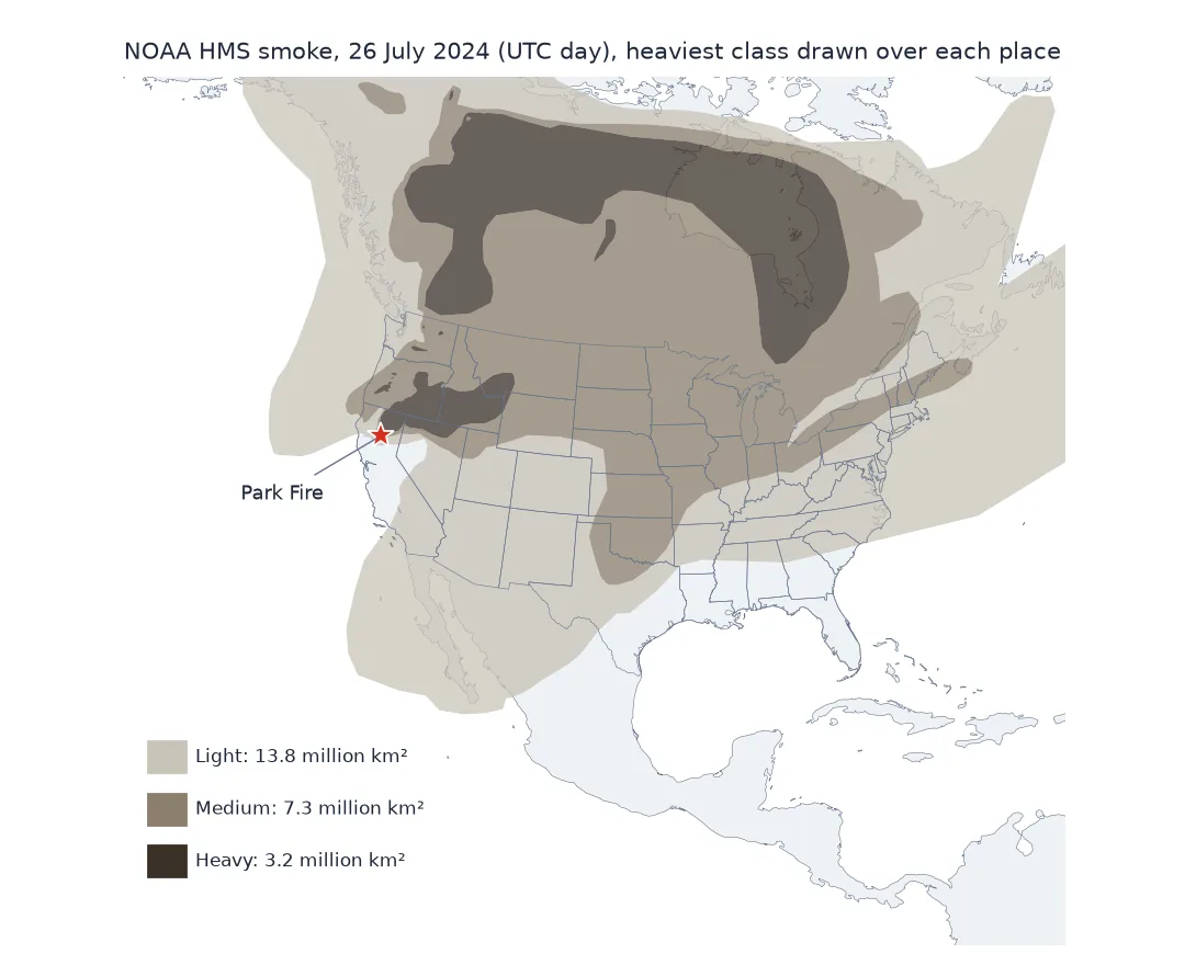
Wildfire smoke reaches far beyond the fire. NOAA's Hazard Mapping System (HMS) analysts outline it every day from satellite imagery: polygons of light, medium and heavy smoke over North America, each tied to the time window in which it was drawn. The polygons are the standard open source for "where was the smoke today" maps, and for estimating who was under it. They need care. Polygons of different densities, and of the same density from different time windows, overlap. Summing their areas counts the same sky several times. And a smoke polygon describes the whole air column seen from space, not what people breathe at ground level.
This page maps HMS smoke over the western United States during the first days of the 2024 Park Fire and measures how much area each density covered without double counting.
Quick answer
Read a day's polygons, project them to an equal-area CRS, and dissolve by density so overlaps count once. For a map where heavier smoke wins, subtract heavier areas from lighter ones:
day = smoke_for(pd.Timestamp("2024-07-26"))
by = {d: day[day.Density == d].union_all() for d in ("Heavy", "Medium", "Light")}
flat = {"Heavy": by["Heavy"], "Medium": by["Medium"].difference(by["Heavy"]),
        "Light": by["Light"].difference(by["Medium"]).difference(by["Heavy"])}
areas = {d: g.area / 1e6 for d, g in flat.items()}
print(f"{len(day)} polygons on 26 Jul 2024 (UTC day); area by heaviest smoke overhead:",
      {d: f"{a:,.0f} km²" for d, a in areas.items()})
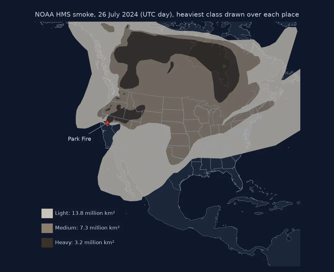
25 polygons on 26 Jul 2024 (UTC day); area by heaviest smoke overhead: {'Heavy': '3,208,848 km²', 'Medium': '7,280,577 km²', 'Light': '13,841,588 km²'}
Polygons and times, no added overlaps, several days
1. Read the polygons and their times
Each polygon records the satellite, the start and end of its analysis window (YYYYDDD HHMM, UTC) and a density class:
print(day[["Satellite", "Start", "End", "Density"]].head(4).to_string(index=False))
print(day.Density.value_counts().to_string())
print(f"analysis windows from {day.Start.min()} to {day.End.max()} (UTC)")
Satellite Start End Density
GOES-EAST 2024208 1451 2024208 1651 Light
GOES-EAST 2024208 1210 2024208 1500 Light
GOES-EAST 2024208 1500 2024208 2320 Light
GOES-EAST 2024208 1210 2024208 1500 Medium
Density
Heavy 15
Medium 7
Light 3
analysis windows from 2024208 1210 to 2024208 2320 (UTC)
2. Do not add overlapping polygons
Analysts draw smoke for several time windows in a day, so polygons overlap heavily. Compare the naive sum of areas with the dissolved area:
naive = day.area.sum() / 1e6
union = day.union_all().area / 1e6
print(f"sum of polygon areas: {naive:,.0f} km²; area under any smoke: {union:,.0f} km² ({naive / union:.1f}x double counting)")
sum of polygon areas: 64,875,908 km²; area under any smoke: 24,331,013 km² (2.7x double counting)
3. Follow the smoke over several days
Repeat the dissolved areas for each day of the fire's first week:
rows = []
for d in DAYS:
    g = smoke_for(d)
    h = g[g.Density == "Heavy"].union_all()
    rows.append({"day": f"{d:%d %b}", "polygons": len(g), "any smoke km²": g.union_all().area / 1e6,
                 "heavy km²": h.area / 1e6 if not h.is_empty else 0})
print(pd.DataFrame(rows).to_string(index=False, float_format="{:,.0f}".format))
day polygons any smoke km² heavy km²
24 Jul 8 32,012,096 6,123,952
25 Jul 14 31,466,623 5,946,625
26 Jul 25 24,331,013 3,208,848
27 Jul 28 28,496,351 4,447,723
Which states were under heavy smoke
The data used on this page
NOAA Hazard Mapping System smoke polygons (daily shapefiles, 24–27 July 2024, UTC days) projected to CONUS Albers (EPSG:5070), state outlines from the 2023 Census cartographic boundary files, and the Park Fire perimeter from CAL FIRE.
from pathlib import Path

import geopandas as gpd
import pandas as pd
import requests

Path("data").mkdir(exist_ok=True)
DAYS = pd.date_range("2024-07-24", "2024-07-27")
URL = "https://satepsanone.nesdis.noaa.gov/pub/FIRE/web/HMS/Smoke_Polygons/Shapefile/"


def smoke_for(d):
    f = Path(f"data/hms_smoke{d:%Y%m%d}.zip")
    if not f.exists():
        f.write_bytes(requests.get(f"{URL}{d:%Y/%m}/{f.name}", timeout=120).content)
    g = gpd.read_file(f).to_crs(5070)
    g["geometry"] = g.geometry.make_valid()
    return g


if not Path("data/cb_2023_us_state_20m.zip").exists():
    Path("data/cb_2023_us_state_20m.zip").write_bytes(requests.get("https://www2.census.gov/geo/tiger/GENZ2023/shp/cb_2023_us_state_20m.zip", timeout=300).content)
STATES = gpd.read_file("data/cb_2023_us_state_20m.zip").query("STUSPS not in ['AK', 'HI', 'PR']").to_crs(5070)
perims = gpd.read_file(requests.get("https://services1.arcgis.com/jUJYIo9tSA7EHvfZ/arcgis/rest/services/California_Fire_Perimeters_last_5_years_View/FeatureServer/0/query",
                                    params={"where": "FIRE_NAME='PARK' AND YEAR_=2024", "outFields": "FIRE_NAME", "outSR": 4326, "f": "geojson"}, timeout=120).text)
PARK = perims.to_crs(5070).geometry.make_valid().union_all()
print(f"{len(DAYS)} days of HMS smoke; Park Fire {PARK.area / 1e6:,.0f} km²")
4 days of HMS smoke; Park Fire 1,739 km²
Example 1: which states were under heavy smoke
heavy = flat["Heavy"]
share = STATES.assign(km2=STATES.area / 1e6, heavy=STATES.geometry.intersection(heavy).area / 1e6)
share["pct"] = share.heavy / share.km2
print(share[share.pct > 0.01].sort_values("pct", ascending=False)[["NAME", "pct"]].head(6).to_string(index=False, formatters={"pct": "{:.0%}".format}))
NAME pct
Idaho 55%
Oregon 38%
Nevada 13%
Montana 10%
California 8%
Washington 3%
An analyst's drawing of a plume
HMS smoke polygons are an analyst's drawing of what satellite imagery shows: the outline of a plume, graded by how opaque it looks. They are drawn in time windows, so a day's file holds several snapshots of plumes that drift and grow, and they overlap. Dissolving by density turns the snapshots into one footprint per class. Subtracting heavier classes from lighter ones gives a map where each place is coloured by the heaviest smoke drawn over it that day.
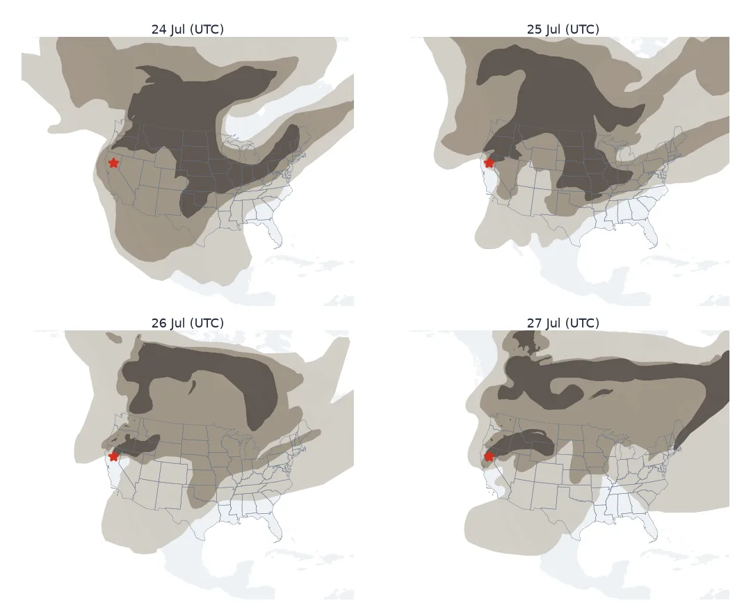
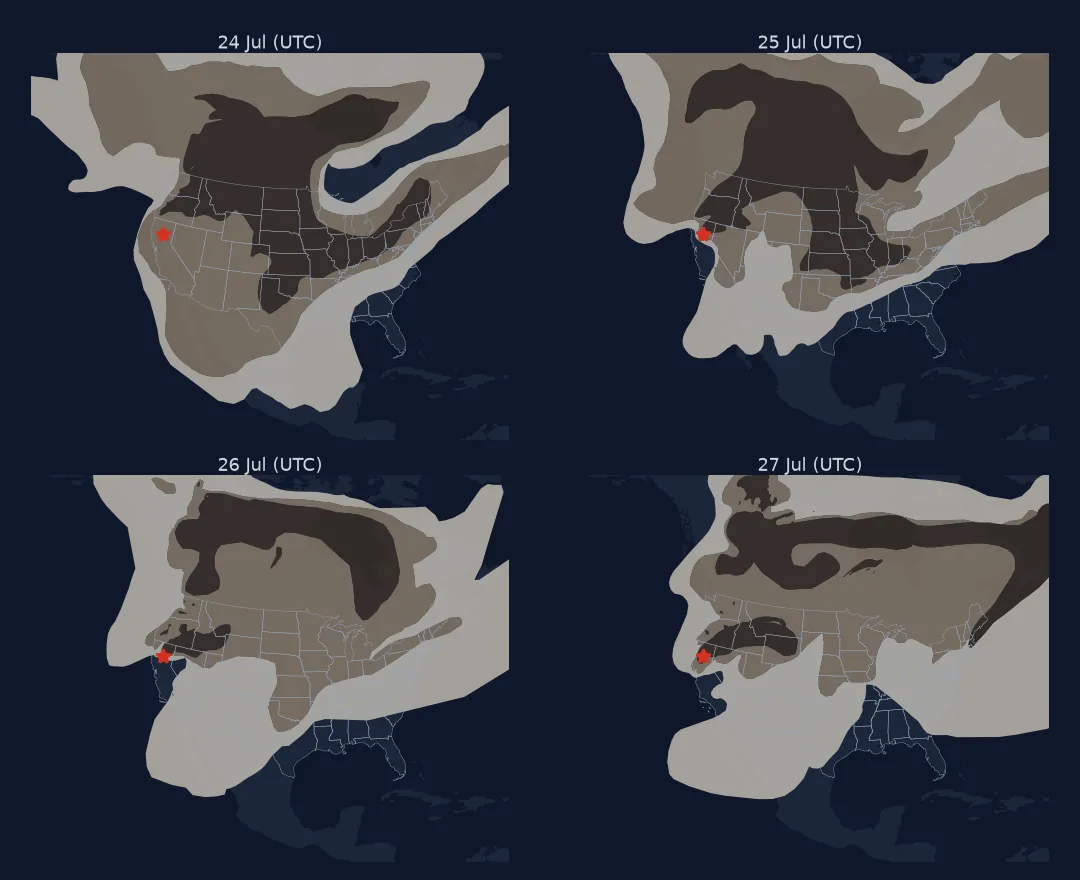
The polygons describe the whole column of air, seen from above. Smoke aloft can pass over a city without affecting the air at the ground, and ground-level smoke under cloud cannot be seen at all. HMS smoke is therefore a map of where smoke was present in the atmosphere, not of air quality. For exposure, combine it with ground monitors (PM2.5) or use it as one indicator among several. The footprint, though, puts a fire in proportion: the Park Fire's burned area is tiny next to the area its smoke, and that of other fires burning at the same time, covered.
Daylight only, several fires and missing days
- Daylight only: analysts draw smoke from visible imagery, so a day's file holds daytime analysis windows within that UTC date. On 26 July they ran from 12:10 to 23:20 UTC, 05:10 to 16:20 Pacific time; smoke at night is not drawn.
- Several fires contribute to the same plumes; HMS does not attribute smoke to a fire.
- Missing days happen when analysts cannot work or imagery is unavailable; check that every day has a file.
- Invalid polygons occur occasionally;
make_valid()before dissolving. - Density classes are qualitative, based on visible opacity; they correspond only loosely to concentrations.
Internal links
- How to use NOAA HMS fire points — the fire detections in the same product
- How to estimate population under smoke — exposure from these polygons
FAQ
Where can I get daily wildfire smoke maps?
NOAA's Hazard Mapping System publishes daily smoke polygons for North America as shapefiles and KML, with light, medium and heavy density classes.
How do I avoid double counting overlapping smoke polygons?
Dissolve the polygons (union_all()) by density class, and subtract heavier classes from lighter ones for a single map.
Does HMS smoke show air quality?
No. It shows smoke in the atmospheric column seen by satellite; ground-level air quality needs monitors such as PM2.5 sensors.
What do HMS smoke density classes mean?
Light, medium and heavy are analyst judgements of visible smoke opacity, roughly increasing with smoke concentration in the column.