How to Map a Wildfire's Daily Progression from Satellite Detections in Python

On this page

Problem statement

A final perimeter shows where a fire burned, not when. A progression map adds the time: the fire's extent at the end of each day, drawn as nested bands. Agencies build them from nightly infrared flights. Where those are not public, satellite fire detections give a usable approximation. Every detection has a time, so the first time each piece of ground was flagged as burning says roughly when the fire reached it. The approximation has rules. Detections are coarse pixels, so the bands must be clipped to a real perimeter. Clouds and smoke delay some first detections. And the band edges are no more precise than a pixel.

This page builds a progression map of the first two and a half days of the 2024 Park Fire from GOES-18 detections and measures how fast it grew.

Quick answer

Give every fire pixel the time it was first detected. For each cut-off time, take the pixels seen so far, turn them into an area, and clip that area to the final perimeter:

first = pts.sort_values("time").drop_duplicates(["lon", "lat"])
first["cell"] = gpd.GeoSeries([CELL[(j, i)] for j, i in zip(first.j, first.i)], index=first.index, crs=3310)
cuts = pd.date_range("2024-07-25 05:00", "2024-07-26 17:00", freq="12h", tz="America/Los_Angeles")   # scans end 16:46 on 26 Jul
bands = []
for c in cuts:
    seen = first[first.time <= c]
    burned = seen.cell.union_all().intersection(PARK)                                 # pixel footprints, clipped
    bands.append((c, burned))
prog = gpd.GeoDataFrame({"until": [c for c, _ in bands]}, geometry=[g for _, g in bands], crs=3310)
prog["km2"] = prog.area / 1e6
print(prog.assign(until=prog.until.dt.strftime("%d %b %H:%M"))[["until", "km2"]].round(0).to_string(index=False))

       until    km2
25 Jul 05:00  366.0
25 Jul 17:00  690.0
26 Jul 05:00  902.0
26 Jul 17:00 1207.0

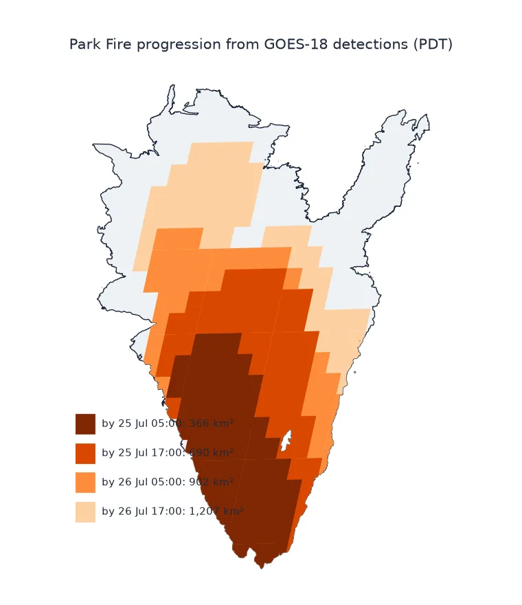
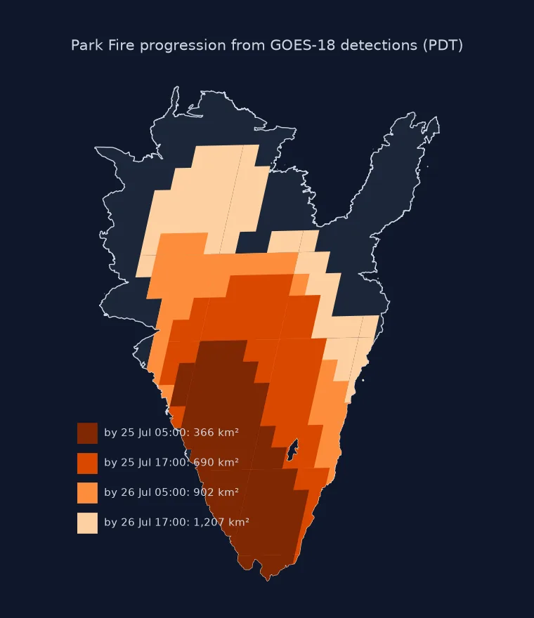
Map of the Park Fire perimeter with nested bands built from GOES-18 pixel footprints: dark brown at the southern end by 05:00 on 25 July, then orange bands further north by 17:00 on 25 July and 05:00 on 26 July, and pale bands in the north by 17:00 on 26 July; the north-east arm and northern edge stay outside the bands. — The Park Fire's first two and a half days from GOES-18 detections, clipped to the final perimeter: 366 km² by the first morning, 1,207 km² by the evening of 26 July.

First detection per pixel, real footprints, growth

1. Take the first detection of each pixel

A burning pixel is flagged in many scans. Only the first matters for progression:

print(f"{len(pts):,} detections, {len(first)} distinct pixels; first at {first.time.min():%d %b %H:%M %Z}, last new pixel at {first.time.max():%d %b %H:%M %Z}")

6,535 detections, 201 distinct pixels; first at 24 Jul 14:46 PDT, last new pixel at 26 Jul 16:46 PDT

2. Use each pixel's real footprint

Each detection is the centre of a pixel. A pixel is a rectangle in the satellite's own projection, but projected onto the ground at California's latitude it is not square: here it is taller north–south than wide east–west. A square buffer around the centre leaves gaps between rows of pixels. Instead, build each pixel's footprint from its four corners in the satellite projection, then clip to the final perimeter to remove the ground the pixels cover but the fire never reached:

w = [c.bounds[2] - c.bounds[0] for c in first.cell]; h = [c.bounds[3] - c.bounds[1] for c in first.cell]
print(f"pixel footprint near the fire: {np.median(w) / 1000:.2f} km east-west x {np.median(h) / 1000:.2f} km north-south")
raw_union = first.cell.union_all()
print(f"pixel footprints: {raw_union.area / 1e6:,.0f} km²; after clipping to the perimeter: {raw_union.intersection(PARK).area / 1e6:,.0f} km² "
      f"(the final perimeter is {PARK.area / 1e6:,.0f} km²)")

pixel footprint near the fire: 2.90 km east-west x 3.10 km north-south
pixel footprints: 1,361 km²; after clipping to the perimeter: 1,207 km² (the final perimeter is 1,739 km²)

3. Measure the growth

The difference between successive bands is the area that first burned in each period, and dividing by the period gives a growth rate:

prog["new_km2"] = prog.km2.diff().fillna(prog.km2.iloc[0])
start = first.time.min()
prog["hours"] = (prog.until - start).dt.total_seconds() / 3600
prog["period_h"] = prog.hours.diff().fillna(prog.hours.iloc[0])                    # the first period starts at the first detection
prog["ha_per_h"] = prog.new_km2 * 100 / prog.period_h
print(prog.assign(until=prog.until.dt.strftime("%d %b %H:%M"))[["until", "period_h", "new_km2", "ha_per_h"]].round(0).to_string(index=False))

       until  period_h  new_km2  ha_per_h
25 Jul 05:00      14.0    366.0    2573.0
25 Jul 17:00      12.0    324.0    2701.0
26 Jul 05:00      12.0    212.0    1763.0
26 Jul 17:00      12.0    306.0    2547.0

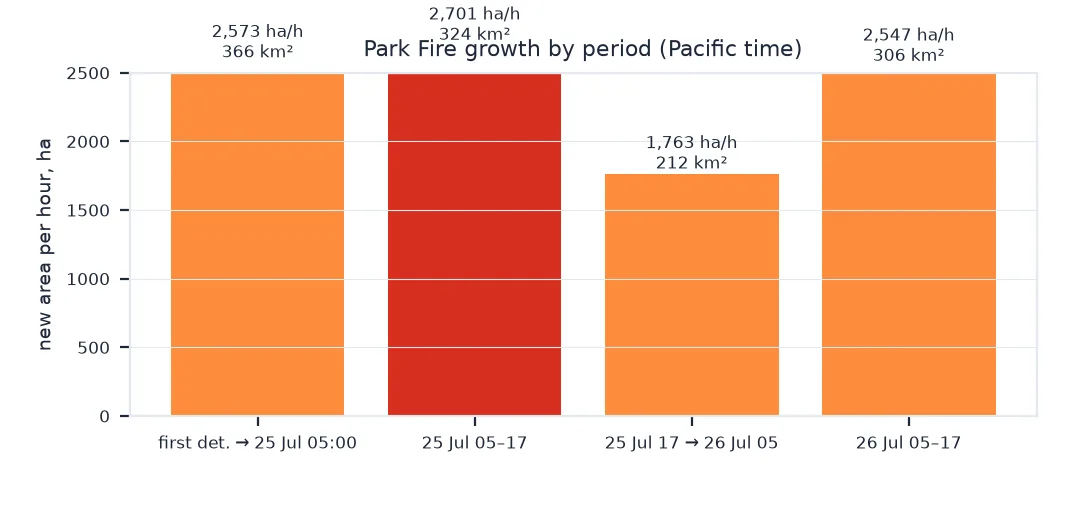
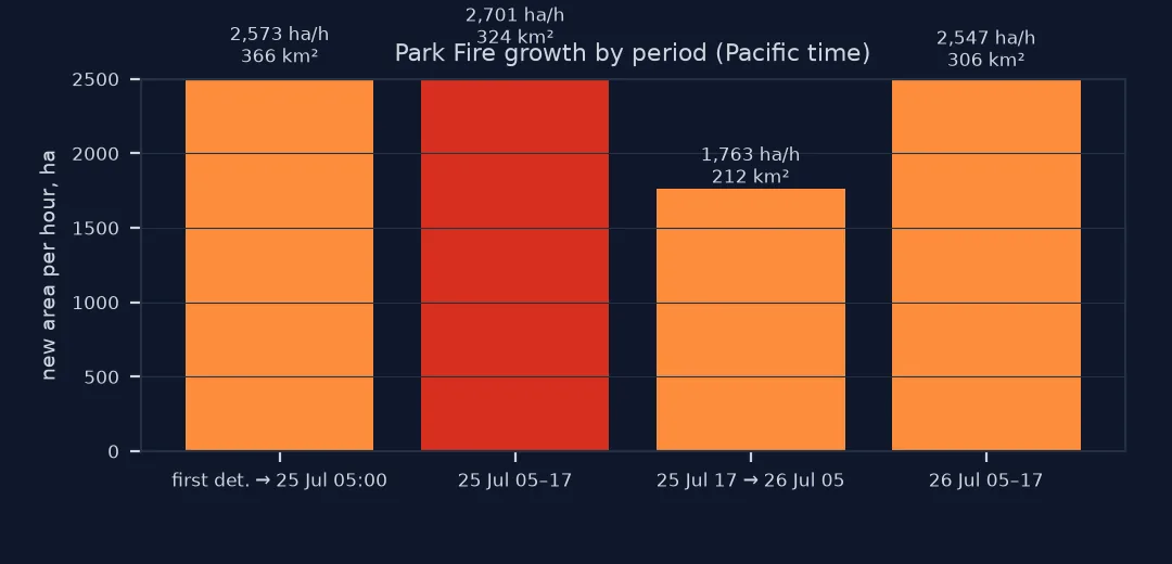
Bar chart of new burned area per hour by period: 2,573 hectares per hour from the first detection to 05:00 on 25 July, 2,701 from 05:00 to 17:00 on 25 July, 1,763 overnight and 2,547 on 26 July. — Growth by period. The overnight period was the slowest; the daytime runs added 2,500 to 2,700 hectares an hour.

A progression saved for a web map

The data used on this page

GOES-18 ABI L2 Fire - Hot Spot Characterization (ABI-L2-FDCC) from NOAA on AWS, one scan per 15 minutes, 21:00 UTC 24 July to 23:45 UTC 26 July 2024; Park Fire final perimeter from CAL FIRE's last-five-years service. Positions are projected to California Albers (EPSG:3310).

import re
from pathlib import Path

import geopandas as gpd
import numpy as np
import pandas as pd
import requests
import xarray as xr
from pyproj import Proj
from shapely.geometry import Polygon

Path("data/fdc").mkdir(parents=True, exist_ok=True)
B = "https://noaa-goes18.s3.amazonaws.com/"
keys = []
for day in (206, 207, 208):
    for h in range(21 if day == 206 else 0, 24):
        text = requests.get(B, params={"list-type": 2, "prefix": f"ABI-L2-FDCC/2024/{day}/{h:02d}/"}, timeout=60).text
        keys += [k for k in re.findall(r"<Key>([^<]+)</Key>", text) if int(re.search(r"_s\d{9}(\d{2})", k).group(1)) % 15 < 5]
FILES = []
for k in keys:
    f = Path("data/fdc", k.rsplit("/", 1)[1])
    if not f.exists():
        f.write_bytes(requests.get(B + k, timeout=120).content)
    FILES.append(f)
with xr.open_dataset(FILES[0], engine="h5netcdf") as ds:
    p = ds.goes_imager_projection
    meanings = dict(zip(ds.Mask.attrs["flag_values"].tolist(), ds.Mask.attrs["flag_meanings"].split()))
    proj = Proj(proj="geos", h=p.perspective_point_height, lon_0=p.longitude_of_projection_origin, sweep=p.sweep_angle_axis,
                a=p.semi_major_axis, b=p.semi_minor_axis)
    x, y = ds.x.values * p.perspective_point_height, ds.y.values * p.perspective_point_height
fire_codes = [c for c, n in meanings.items() if n.endswith("fire_pixel") and "no_fire" not in n]
bx, by = proj([-122.3, -121.3, -122.3, -121.3], [39.6, 39.6, 40.5, 40.5])
IX, IY = (x >= min(bx)) & (x <= max(bx)), (y >= min(by)) & (y <= max(by))
LON, LAT = proj(*np.meshgrid(x[IX], y[IY]), inverse=True)
rows = []
for f in FILES:
    with xr.open_dataset(f, engine="h5netcdf") as ds:
        m = ds.Mask.values[np.ix_(IY, IX)]
        t = pd.Timestamp(ds.attrs["time_coverage_start"].rstrip("Z"), tz="UTC")
        for j, i in zip(*np.nonzero(np.isin(m, fire_codes))):
            rows.append((t, LON[j, i], LAT[j, i], j, i))
det = pd.DataFrame(rows, columns=["time", "lon", "lat", "j", "i"])
det["time"] = det.time.dt.tz_convert("America/Los_Angeles")
pts = gpd.GeoDataFrame(det, geometry=gpd.points_from_xy(det.lon, det.lat), crs=4326).to_crs(3310)
perims = gpd.read_file(requests.get("https://services1.arcgis.com/jUJYIo9tSA7EHvfZ/arcgis/rest/services/California_Fire_Perimeters_last_5_years_View/FeatureServer/0/query",
                                    params={"where": "FIRE_NAME='PARK' AND YEAR_=2024", "outFields": "FIRE_NAME", "outSR": 4326, "f": "geojson"}, timeout=120).text)
PARK = perims.to_crs(3310).geometry.make_valid().union_all()
xs, ys = x[IX], y[IY]
dx, dy = abs(xs[1] - xs[0]), abs(ys[1] - ys[0])
CELL = {}
for j, i in set(zip(det.j, det.i)):                                              # footprint of each fire pixel
    cx = [xs[i] - dx / 2, xs[i] + dx / 2, xs[i] + dx / 2, xs[i] - dx / 2]
    cy = [ys[j] - dy / 2, ys[j] - dy / 2, ys[j] + dy / 2, ys[j] + dy / 2]
    lon, lat = proj(cx, cy, inverse=True)
    CELL[(j, i)] = gpd.GeoSeries([Polygon(zip(lon, lat))], crs=4326).to_crs(3310).iloc[0]
print(f"{len(pts):,} fire detections in {len(CELL)} distinct pixels")

6,535 fire detections in 201 distinct pixels

Example 1: save the progression for a web map

out = prog.to_crs(4326).assign(until=prog.until.dt.strftime("%Y-%m-%dT%H:%M%z"))
out.to_file("data/park_progression.geojson", driver="GeoJSON")
print(f"{len(out)} progression polygons written, {Path('data/park_progression.geojson').stat().st_size / 1e3:.0f} kB")

4 progression polygons written, 965 kB

Detections give times, perimeters give shape

A progression map is a sequence of cumulative areas: everything burned by each cut-off time. Satellite detections supply the times; the final perimeter supplies the shape. Neither alone is enough. The detections are too coarse to draw an edge, and the perimeter has no time at all. Combining them gives bands whose timing comes from the satellite and whose outline comes from the ground and air mapping.

From detections to a progression map.

The result is approximate in known ways. A pixel is flagged once enough of it burns hot, so a band edge can be a pixel early or late. A pixel hidden by smoke or cloud is first seen late, which pushes ground into a later band than it belongs. And by the evening of 26 July the bands cover 1,207 km², about 70% of the final perimeter. The rest is ground that burned later, plus ground the 3 km pixels never flagged. The growth figures are still informative: they show when the fire made its runs and how large each one was.

Local time, agency progressions and spot fires

Progression mapping problems and fixes.

Local time: cut-offs here are 05:00 and 17:00 Pacific time, near the daily low and high of fire activity.
Better detections: VIIRS (375 m) from polar orbiters gives finer pixels but only a few passes a day; combining both is common.
Agency progressions: where infrared perimeter flights are published (NIFC, incident sites), use them for the shape of each day.
Spot fires ahead of the front appear as isolated pixels; the union keeps them as separate bits of each band.
Pixel shape changes across the satellite's view; build footprints from the pixel corners, as the setup does, rather than assuming squares.

Internal links

How to track a wildfire with GOES detections — the detections used here
How to download CAL FIRE perimeters — the final perimeter

FAQ

How do I make a fire progression map?

Take the time each location first burned (from detections or nightly perimeters), and for each cut-off time map the area burned by then; draw the cumulative areas as nested bands.

Can satellite fire detections show fire spread?

Yes, approximately: the first time each pixel is detected marks when the fire reached it, to within a scan interval and a pixel.

Why clip detections to the final perimeter?

Detection pixels are kilometres across and cover unburned ground at the fire's edge; the perimeter removes it.

What is a fire run?

A period of rapid spread, usually in the afternoon heat and wind; progression maps show runs as wide bands between cut-off times.