How to Estimate How Many People Were Under Wildfire Smoke in Python

On this page

Problem statement

"Smoke affected 100 million people" is the kind of number reported every fire season. It comes from overlaying smoke plumes with population, and the method behind it changes the answer. The smoke polygons are huge and coarse, population comes in census units, and the two never line up. Assign each county wholly to the smoke class at its centroid, or split its population by the share of its area under smoke? Count a county once, under the heaviest smoke drawn over it, or under every overlapping polygon? Each choice moves the total by millions.

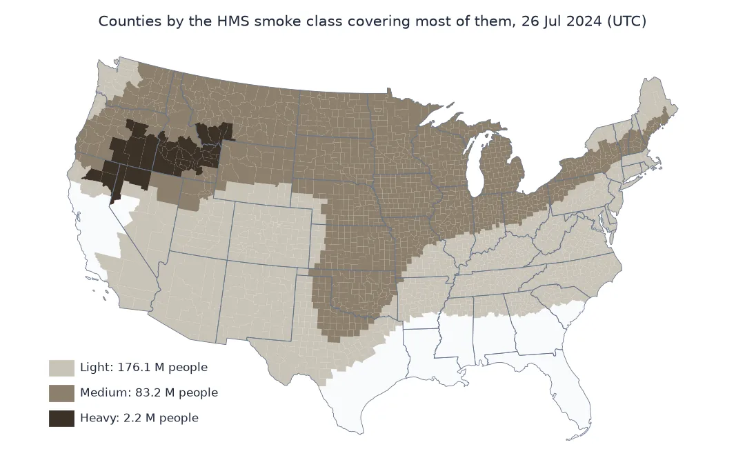
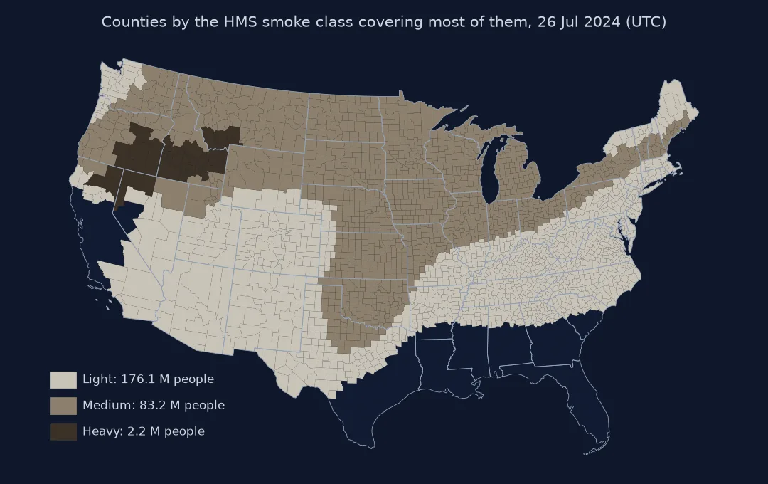
This page estimates how many people in the contiguous United States were under each class of NOAA HMS smoke on 26 July 2024, during the first days of the Park Fire. It compares two allocation methods.

Quick answer

Dissolve the smoke by heaviest class, intersect it with county polygons, and allocate each county's population by the share of its area in each class:

pieces = gpd.overlay(COUNTIES[["GEOID", "pop", "area_km2", "geometry"]], SMOKE[["density", "geometry"]], how="intersection")
pieces["people"] = pieces["pop"] * (pieces.area / 1e6) / pieces.area_km2
area_weighted = pieces.groupby("density").people.sum().reindex(["Heavy", "Medium", "Light"])
print((area_weighted / 1e6).round(1).to_string(), f"\nanywhere under smoke: {area_weighted.sum() / 1e6:.1f} million of {COUNTIES['pop'].sum() / 1e6:.1f} million")

density
Heavy       2.2
Medium     83.2
Light     176.1 
anywhere under smoke: 261.5 million of 332.7 million

Map of the contiguous United States with counties coloured by the HMS smoke class covering most of each on 26 July 2024: heavy smoke over Idaho, eastern Oregon and northern Nevada; medium smoke across the northern tier from Washington to New England and down through the Plains; light smoke over most of the South and West; California's coast and the Gulf Coast states largely clear. — Counties by the smoke class over most of their area. By area-weighted population, 2.2 million people were under heavy smoke, 83 million under medium and 176 million under light.

Flatten the smoke, then weight by area

1. Flatten the smoke first

HMS polygons of different densities and time windows overlap. Without flattening, a county under three polygons would be counted three times. Keep only the heaviest class at each place:

print(SMOKE.assign(km2=SMOKE.area / 1e6)[["density", "km2"]].to_string(index=False, float_format="{:,.0f}".format))
print(f"overlap between classes after flattening: {SMOKE.geometry.iloc[0].intersection(SMOKE.geometry.iloc[1]).area:.0f} m²")

density        km2
  Heavy  3,208,848
 Medium  7,280,577
  Light 13,841,588
overlap between classes after flattening: 0 m²

2. Compare with centroid assignment

The quick way gives each county wholly to the class at its centroid. Compare the two methods:

cent = COUNTIES.set_geometry(COUNTIES.representative_point())
joined = gpd.sjoin(cent, SMOKE[["density", "geometry"]], how="left", predicate="within")
centroid = joined.groupby("density")["pop"].sum().reindex(["Heavy", "Medium", "Light"])
cmp = pd.DataFrame({"area-weighted (M)": area_weighted / 1e6, "centroid (M)": centroid / 1e6})
cmp["difference"] = cmp["centroid (M)"] - cmp["area-weighted (M)"]
print(cmp.round(2).to_string())

         area-weighted (M)  centroid (M)  difference
density                                             
Heavy                 2.24          2.13       -0.12
Medium               83.16         83.34        0.18
Light               176.08        175.21       -0.87

The two allocation methods agree closely with plumes this large.

3. See who was under heavy smoke

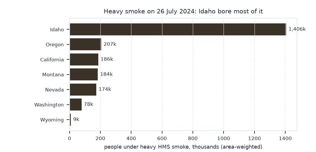
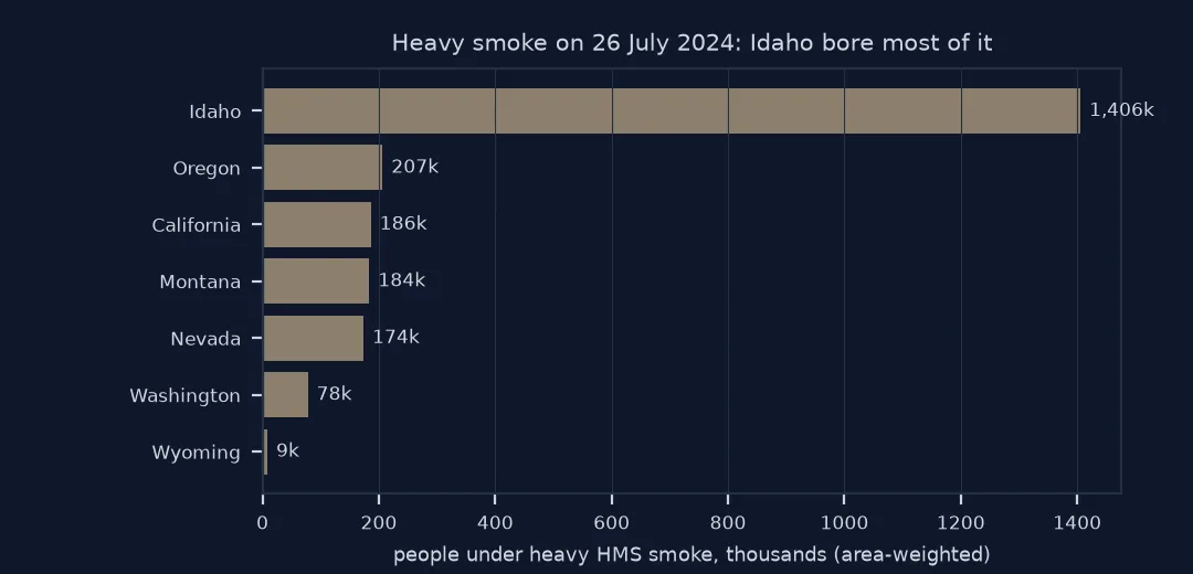
Rank states by the population under heavy smoke:

heavy = pieces[pieces.density == "Heavy"].groupby(pieces.GEOID.str[:2]).people.sum()
top = heavy.rename(STATE_NAME).sort_values(ascending=False).head(5)
print((top / 1e3).round(0).astype(int).astype(str).add(" thousand").to_string())

GEOID
Idaho         1406 thousand
Oregon         207 thousand
California     186 thousand
Montana        184 thousand
Nevada         174 thousand

Each state's share of people under smoke

The data used on this page

NOAA Hazard Mapping System smoke polygons for 26 July 2024 (UTC day); county outlines (2023 cartographic boundary files) and county population estimates for 1 July 2023 (vintage 2023) from the US Census Bureau, in CONUS Albers (EPSG:5070).

from pathlib import Path

import geopandas as gpd
import pandas as pd
import requests

Path("data").mkdir(exist_ok=True)
SRC = {"hms_smoke20240726.zip": "https://satepsanone.nesdis.noaa.gov/pub/FIRE/web/HMS/Smoke_Polygons/Shapefile/2024/07/hms_smoke20240726.zip",
       "cb_2023_us_county_20m.zip": "https://www2.census.gov/geo/tiger/GENZ2023/shp/cb_2023_us_county_20m.zip",
       "co-est2023-alldata.csv": "https://www2.census.gov/programs-surveys/popest/datasets/2020-2023/counties/totals/co-est2023-alldata.csv"}
for name, url in SRC.items():
    if not Path("data", name).exists():
        Path("data", name).write_bytes(requests.get(url, timeout=600).content)
raw = gpd.read_file("data/hms_smoke20240726.zip").to_crs(5070)
raw["geometry"] = raw.geometry.make_valid()
u = {d: raw[raw.Density == d].union_all() for d in ("Heavy", "Medium", "Light")}
flat = {"Heavy": u["Heavy"], "Medium": u["Medium"].difference(u["Heavy"]), "Light": u["Light"].difference(u["Medium"]).difference(u["Heavy"])}
SMOKE = gpd.GeoDataFrame({"density": list(flat)}, geometry=list(flat.values()), crs=5070)
pe = pd.read_csv("data/co-est2023-alldata.csv", encoding="latin-1", dtype={"STATE": str, "COUNTY": str}).query("SUMLEV == 50")
pop = pd.Series(pe.POPESTIMATE2023.to_numpy(), index=pe.STATE + pe.COUNTY)
COUNTIES = gpd.read_file("data/cb_2023_us_county_20m.zip").query("STUSPS not in ['AK', 'HI', 'PR']").to_crs(5070)
COUNTIES["pop"] = COUNTIES.GEOID.map(pop)
COUNTIES = COUNTIES.dropna(subset=["pop"])
COUNTIES["area_km2"] = COUNTIES.area / 1e6
STATE_NAME = dict(zip(pe.STATE, pe.STNAME))
print(f"{len(COUNTIES):,} counties with 2023 population, {COUNTIES['pop'].sum() / 1e6:.1f} million people")

3,109 counties with 2023 population, 332.7 million people

any_smoke = pieces.groupby(pieces.GEOID.str[:2]).people.sum()
state_pop = COUNTIES.groupby(COUNTIES.GEOID.str[:2])["pop"].sum()
share = (any_smoke.reindex(state_pop.index).fillna(0) / state_pop).rename(STATE_NAME).sort_values()
print("lowest:", ", ".join(f"{k} {v:.1%}" for k, v in share.head(3).items()))
print("highest:", ", ".join(f"{k} {v:.0%}" for k, v in share.tail(3).items()))

lowest: Louisiana 0.0%, Florida 0.0%, Mississippi 25.7%
highest: District of Columbia 100%, Washington 100%, West Virginia 100%

Exposure is areal interpolation

Exposure estimates like these are areal interpolation: population is known for counties, smoke for polygons that ignore county lines. Area weighting assumes people are spread evenly within each county, which is wrong in detail but unbiased overall. Centroid assignment assumes everyone lives at one point, which is fine for small counties and badly wrong for large western counties that straddle a smoke edge. With continent-sized smoke polygons the two methods agree on the total, because most counties lie wholly inside or outside a class. They differ for the counties on the edges.

Horizontal bar chart of people under heavy smoke by state on 26 July 2024: Idaho about 1.4 million, then Oregon, California, Montana and Nevada around 170,000 to 210,000 each. — Heavy smoke was concentrated: Idaho alone had more people under it than every other state together.

Two caveats belong next to any such number. HMS smoke is column smoke seen from space, not air quality at the ground. "Under heavy smoke" means a satellite saw thick smoke overhead, which may or may not have reached street level. And the count describes one UTC day. Exposure over a fire season sums days, and should weight them by measured PM2.5 where possible.

Dasymetric refinement and daylight windows

Exposure problems and fixes.

Dasymetric refinement: weighting by a population grid (GHSL, WorldPop) or census blocks instead of evenly spread county population sharpens edge counties.
Connecticut uses planning regions in the 2023 files; they match the 2023 outlines used here.
Flatten first: overlapping polygons must be dissolved before any overlay, or people are counted once per polygon.
Daylight windows: a day's HMS smoke file holds analysis windows within that UTC date, drawn from daylight imagery.
Ground truth: PM2.5 monitors (AirNow, PurpleAir) measure what people breathed; use them to check exposure claims.

Internal links

How to map smoke plumes from HMS — the polygons and their overlaps
How to map net migration by county — another county-population overlay

FAQ

How do I estimate the population affected by wildfire smoke?

Overlay daily smoke polygons with population data: intersect them with census units and allocate each unit's population by the share of its area under smoke.

What is area-weighted interpolation?

Allocating a value from source zones (counties) to target zones (smoke polygons) in proportion to the overlapping area, assuming the value is spread evenly within each source zone.

Is centroid assignment good enough?

For small units, yes; for large counties on a smoke edge it can put a whole county's population on the wrong side.

Does being under HMS smoke mean breathing smoke?

Not necessarily; HMS shows smoke anywhere in the atmospheric column. Ground-level PM2.5 measurements show what reached people.