How to Delineate an Urban Extent from GHSL in Python

On this page

Problem statement

"The population of Den Haag" and "the density of Den Haag" depend on where Den Haag ends. The municipal boundary is a legal line that includes dunes, sea and farmland in some places and stops mid-street in others, where the city runs on into Rijswijk, Voorburg and Delft without a break. Comparing cities needs a boundary drawn the same way everywhere: from where people and buildings actually are.

The Global Human Settlement Layer publishes population and built-up surface on regular grids for the whole world, and the EU–UN Degree of Urbanisation defines urban centres on them with a simple rule. A simplified version of that rule takes a few dozen lines of Python.

Quick answer

Density threshold, contiguity, population threshold:

import io, zipfile, requests, numpy as np, rasterio, rasterio.features, rasterio.mask, geopandas as gpd
from scipy import ndimage
from shapely.geometry import shape

BASE = "https://jeodpp.jrc.ec.europa.eu/ftp/jrc-opendata/GHSL"
for kind, name in (("POP", "GHS_POP_E2020_GLOBE_R2023A_4326_30ss"),
                   ("BUILT_S", "GHS_BUILT_S_E2020_GLOBE_R2023A_4326_30ss")):
    url = f"{BASE}/GHS_{kind}_GLOBE_R2023A/{name}/V1-0/tiles/{name}_V1_0_R4_C19.zip"
    zipfile.ZipFile(io.BytesIO(requests.get(url, timeout=600).content)).extractall("ghsl_nl")

W, S, E, N = 3.9, 51.8, 4.8, 52.4                      # Den Haag, Rotterdam and surroundings
def read(name):
    with rasterio.open(f"ghsl_nl/{name}_V1_0_R4_C19.tif") as src:
        win = rasterio.windows.from_bounds(W, S, E, N, src.transform)
        return src.read(1, window=win).astype("float64"), src.window_transform(win)
pop, tf = read("GHS_POP_E2020_GLOBE_R2023A_4326_30ss")
built, _ = read("GHS_BUILT_S_E2020_GLOBE_R2023A_4326_30ss")

lat = N - (np.arange(pop.shape[0]) + 0.5) * abs(tf.e)
cell_km2 = np.broadcast_to((abs(tf.a) * 111.32 * np.cos(np.radians(lat))[:, None])
                           * (abs(tf.e) * 110.57), pop.shape)          # km² per cell
density = np.clip(pop, 0, None) / cell_km2                       # people per km²

dense = density >= 1500
labels, n = ndimage.label(dense)                                  # rook contiguity
cluster_pop = ndimage.sum(np.clip(pop, 0, None), labels, index=np.arange(1, n + 1))
centres = np.isin(labels, np.where(cluster_pop >= 50_000)[0] + 1)
print(f"grid: {pop.shape[1]} × {pop.shape[0]} cells of 30 arc-seconds (~{cell_km2.mean():.2f} km²)")
print(f"dense clusters: {n}; urban centres (≥ 50,000 people): {(cluster_pop >= 50_000).sum()}")
for i in np.argsort(cluster_pop)[::-1][:4]:
    m = labels == i + 1
    print(f"  cluster {i + 1}: {cluster_pop[i]:>9,.0f} people on {cell_km2[m].sum():6.1f} km², "
          f"built-up {built[m].sum() / 1e6 / cell_km2[m].sum():.0%} of the land")

grid: 108 × 72 cells of 30 arc-seconds (~0.53 km²)
dense clusters: 106; urban centres (≥ 50,000 people): 10
  cluster 66:   855,655 people on  210.4 km², built-up 25% of the land
  cluster 40:   797,550 people on  120.9 km², built-up 26% of the land
  cluster 28:   253,465 people on   52.4 km², built-up 26% of the land
  cluster 1:   154,526 people on   27.7 km², built-up 26% of the land

The two largest clusters are Rotterdam's (cluster 66, 856,000 people on 210 km²) and Den Haag's (cluster 40, 798,000 on 121 km²). Both ignore municipal boundaries: each takes in the neighbouring municipalities it has grown into, and stops where the density does. Built-up land covers about a quarter of every one of the four largest.

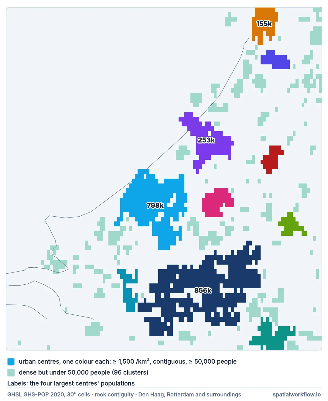
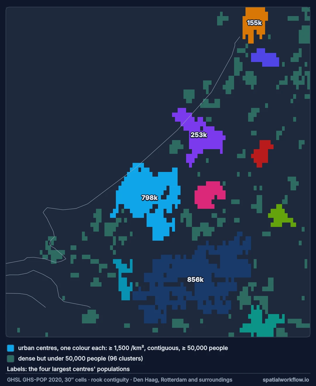
Map of South Holland on a grid of 1 km cells: ten urban centres each in their own colour, the largest being Rotterdam’s in the south with 856,000 people and Den Haag’s on the coast with 798,000; many small dense clusters under 50,000 people in pale green scattered between them. — The three rules from the code above, applied cell by cell. Every coloured patch is one of the 10 urban centres: a contiguous run of cells over 1,500 people per km² holding at least 50,000 people. The pale ones are the other 96 dense clusters, too small to count. Rotterdam’s centre (856,000) and Den Haag’s (798,000) sprawl across several municipalities, and the gap between them is the Midden-Delfland green belt.

Same-epoch grids, densities, a threshold, contiguity

1. Get population and built-up grids for the same epoch

GHS-POP (residents per cell) and GHS-BUILT-S (built-up square metres per cell) share a grid. The 30 arc-second WGS84 version is convenient; the official Degree of Urbanisation uses the 1 km Mollweide grid.

2. Convert counts to densities

Cells in geographic coordinates shrink with latitude. Divide by each row's cell area, not a constant.

3. Apply the density threshold

The Degree of Urbanisation uses 1,500 inhabitants per km² for urban-centre cells (and 300 for urban clusters).

4. Group contiguous cells and apply the population threshold

Label connected dense cells; keep clusters with at least 50,000 people. The official method uses four-neighbour contiguity and fills small gaps; this version keeps only the core steps.

5. Vectorise and compare with administrative boundaries

Turn the kept clusters into polygons and overlay them on municipalities to see how much of each urban centre each municipality holds.

Three thresholds turn a population grid into urban centres drawn the same way everywhere.

Urban centre polygons and built-up share

Example 1 — polygons of the urban centres

shapes = rasterio.features.shapes(labels.astype("int32"), mask=centres, transform=tf)
polys = gpd.GeoDataFrame([{"cluster": int(v), "geometry": shape(g)} for g, v in shapes],
                         crs=4326).dissolve("cluster").reset_index()
polys["people"] = [cluster_pop[c - 1] for c in polys.cluster]
polys["km2"] = polys.to_crs(28992).area / 1e6
polys.to_file("urban_centres.gpkg")
print(polys.sort_values("people", ascending=False)[["cluster", "people", "km2"]]
      .round({"people": -3, "km2": 1}).to_string(index=False))

 cluster   people   km2
      66 856000.0 212.2
      40 798000.0 121.9
      28 253000.0  52.9
       1 155000.0  27.9
      45 128000.0  24.9
      95 125000.0  30.9
      52  68000.0  14.3
      36  65000.0  14.3
      81  58000.0  17.5
       9  54000.0  14.8

These polygons are comparable with urban centres anywhere in the world drawn by the same rule — which is what municipal boundaries are not.

Example 2 — the municipality against the urban centre

import osmnx as ox
ox.settings.http_user_agent = "spatialworkflow-examples/1.0"
gem = ox.geocode_to_gdf("Den Haag, Netherlands").to_crs(4326)
from shapely.geometry import Point
row = polys[polys.contains(Point(4.3113, 52.0799))].iloc[0]           # the centre containing Den Haag
centre, g = row.geometry, gem.geometry.iloc[0]
print(f"clusters containing Den Haag and Rotterdam: {row.cluster}, "
      f"{polys[polys.contains(Point(4.4777, 51.9244))].cluster.tolist()}")
with rasterio.open("ghsl_nl/GHS_POP_E2020_GLOBE_R2023A_4326_30ss_V1_0_R4_C19.tif") as src:
    in_gem, _ = rasterio.mask.mask(src, [g], crop=True, nodata=0)
print(f"municipality: {gem.to_crs(28992).area.iloc[0] / 1e6:.0f} km², "
      f"{np.clip(in_gem, 0, None).sum():,.0f} people")
print(f"Den Haag urban centre: {row.km2:.0f} km², {row.people:,.0f} people")
inside = gpd.GeoSeries([centre.intersection(g)], crs=4326).to_crs(28992).area.iloc[0] / 1e6
print(f"share of the urban centre inside the municipality: {inside / row.km2:.0%}; "
      f"share of the municipality inside the urban centre: {inside / (gem.to_crs(28992).area.iloc[0] / 1e6):.0%}")

clusters containing Den Haag and Rotterdam: 40, [66]
municipality: 98 km², 550,960 people
Den Haag urban centre: 122 km², 797,550 people
share of the urban centre inside the municipality: 56%; share of the municipality inside the urban centre: 69%

The two shapes overlap only in part. Den Haag's urban centre holds nearly 250,000 more people than the municipality, and only 56% of its area lies inside it — the rest is the neighbouring towns it has merged with. A third of the municipality lies outside the centre: dunes, beach and parkland below the density threshold. Densities computed on either are real numbers; they are numbers about different objects.

from pyproj import Geod
geod = Geod(ellps="WGS84")
rows, cols = np.indices(pop.shape)
lons, lats = rasterio.transform.xy(tf, rows.ravel(), cols.ravel())
_, _, dist = geod.inv(np.full(len(lons), 4.3113), np.full(len(lats), 52.0799), lons, lats)
dist_km = (np.array(dist) / 1000).reshape(pop.shape)
share = built / (cell_km2 * 1e6)
for lo, hi in ((0, 2), (2, 5), (5, 10), (10, 20), (20, 30)):
    ring = (dist_km >= lo) & (dist_km < hi)
    print(f"{lo:>2}–{hi:<2} km: built-up {share[ring].mean():5.1%} of the land, "
          f"{np.clip(pop[ring], 0, None).sum() / cell_km2[ring].sum():6,.0f} people/km²")

 0–2  km: built-up 30.9% of the land, 10,892 people/km²
 2–5  km: built-up 19.3% of the land,  5,362 people/km²
 5–10 km: built-up 12.4% of the land,  1,483 people/km²
10–20 km: built-up 10.7% of the land,  1,016 people/km²
20–30 km: built-up  7.2% of the land,    816 people/km²

The gradient from centre to edge is the continuous reality that any boundary cuts. Where on it the line falls decides every density figure computed inside the line.

Density falls continuously; any boundary is a cut through the gradient.

Grid rules, density and contiguity

Why a grid-based definition

A rule applied to a regular grid gives the same answer wherever it is applied, independent of how local government is organised. That is why the Degree of Urbanisation was adopted by the UN Statistical Commission for international comparison, and why its urban centres cross municipal lines freely.

Why density and contiguity

Density picks out cells where people live closely; contiguity joins them into places; the population threshold separates cities from dense villages. Each threshold is a convention, chosen to match what people recognise as a city across very different countries.

Why the simplified version differs from the official one

The official method uses a 1 km equal-area grid, fills gaps in clusters, smooths edges and adds a built-up criterion. A 30 arc-second grid in degrees has cells of about 0.57 km² at this latitude, and skipping gap-filling leaves holes. The result is close in shape and not identical in numbers; for official comparisons, use the published GHS-SMOD layer.

The legal city and the functional one overlap by little more than half.

SMOD, coastal cells and tile edges

GHS-SMOD publishes the official settlement classification directly; use it when the exact method matters.
Coastal cells mix land and sea; densities per cell area understate land density there.
Epochs: GHSL provides 1975–2030 in five-year steps, which makes growth analyses straightforward.
Tile edges: a region near a tile boundary needs two tiles mosaicked.
Negative or no-data values do not occur in GHS-POP 2023 but check older releases.

Internal links

Urban extent explained — administrative, morphological and functional cities
Density depends on the boundary — the fix guide for density comparisons
How to calculate population-weighted exposure — the same population grid, used differently
Modifiable areal unit problem explained — why boundaries move answers
How to clip a raster to a polygon — masking grids by boundaries
Urban morphology explained — form within the extent

FAQ

How do I define a city's boundary from data?

Use a population grid: cells above a density threshold, grouped by contiguity, kept if the group exceeds a population threshold — the Degree of Urbanisation approach.

What is GHSL?

The European Commission's Global Human Settlement Layer: global grids of population, built-up surface and settlement type from 1975 to 2030.

What thresholds define an urban centre?

1,500 people per km² in contiguous 1 km cells totalling at least 50,000 people.

Why does the urban centre cross municipal boundaries?

Because the rule looks at where people live, not at administrative lines.

Should I use my own delineation or GHS-SMOD?

GHS-SMOD for official comparability; your own when you need to vary the thresholds or the grid.

Why is the municipality's density different?

Its area includes non-urban land and excludes parts of the continuous city; it measures a different object.