How to Measure Built-Up Area per Person with GHSL in Python

On this page

Problem statement

Whether a country builds on more land than its population growth needs is a question of two grids: how much surface is built up, and how many people live there. The GHSL publishes both on the same grid for every epoch since 1975, GHS-BUILT-S for built-up surface and GHS-POP for population, which makes built-up area per person, and the UN's land-consumption indicator for Sustainable Development Goal 11.3.1, a few lines of raster arithmetic.

This page sums GHS-BUILT-S and GHS-POP for the Netherlands in 1975 and 2020, computes built-up area per person, the ratio of land consumption rate to population growth rate, and the same by municipality, and checks which places built most per new resident.

Quick answer

Mask both layers with the same boundary and divide the sums:

rows = {}
for y in (1975, 2020):
    b, p = clip(tile("BUILT_S", y), NL).sum(), clip(tile("POP", y), NL).sum()
    rows[y] = (b, p)
    print(f"{y}: built-up {b / 1e6:,.0f} km2, population {p:,.0f}, {b / p:,.0f} m2 per person")
(b0, p0), (b1, p1) = rows[1975], rows[2020]
print(f"1975-2020: built-up {b1 / b0 - 1:+.0%}, population {p1 / p0 - 1:+.0%}")

1975: built-up 952 km2, population 13,634,895, 70 m2 per person
2020: built-up 1,899 km2, population 17,389,161, 109 m2 per person
1975-2020: built-up +99%, population +28%

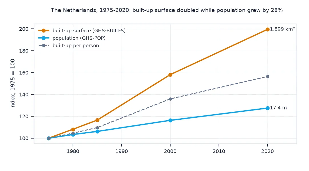
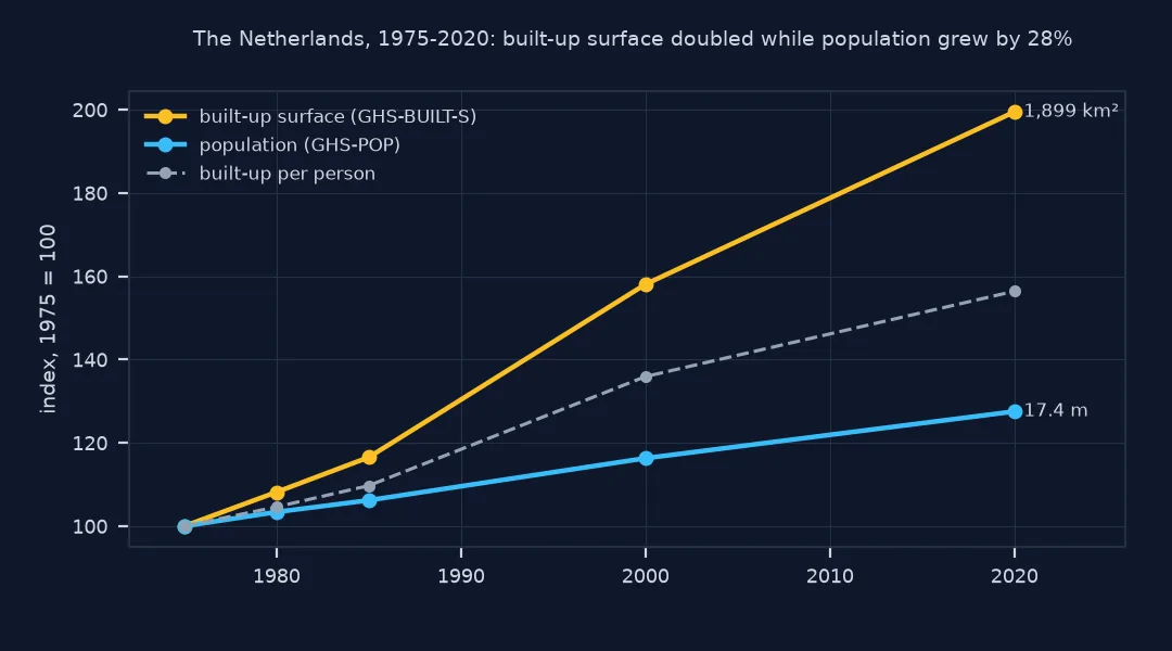
Between 1975 and 2020 the built-up surface of the Netherlands doubled, from 952 to 1,899 km², while the population grew by 28%. Built-up area per person rose from 70 to 109 m².

Line chart indexed to 1975 for the Netherlands: built-up surface rises to 200 by 2020, 1,899 square kilometres; population to 128, 17.4 million; built-up area per person to about 156. — Built-up surface and population since 1975.

What the built-up layer counts, the SDG ratio, municipalities

1. What GHS-BUILT-S counts

Each cell holds the square metres of built-up surface in it, from building footprints and other roofed structures detected in satellite imagery; roads are not included. Look at the values the cells take:

b20 = clip(tile("BUILT_S", 2020), NL)
with rasterio.open(tile("BUILT_S", 2020)) as src:
    print(f"{src.dtypes[0]}, nodata {src.nodata}, {src.res[0] * 3600:.0f} arc-seconds")
v = b20.compressed()
print(f"cells: {v.size:,}; with no built-up surface: {(v == 0).sum():,}; largest {v.max():,.0f} m2")
print(f"built-up share of the land: {v.sum() / 1e6 / NL.area.iloc[0] * 1e6:.1%}")

uint32, nodata None, 30 arc-seconds
cells: 66,490; with no built-up surface: 5,033; largest 452,358 m2
built-up share of the land: 5.4%

The layer is stored as unsigned integers with no nodata value. 5,033 of the 66,490 land cells have no built-up surface; the most built-up cell holds 452,358 m², most of its area. Altogether 5.4% of the land is covered by buildings.

2. The SDG 11.3.1 ratio

The indicator divides the annual rate of land consumption by the annual rate of population growth, both as log rates over the same period. Above 1, built-up area grew faster than population:

yrs = 2020 - 1975
lcr = np.log(b1 / b0) / yrs
pgr = np.log(p1 / p0) / yrs
print(f"land consumption rate {lcr:.4f} per year, population growth rate {pgr:.4f} per year, ratio {lcr / pgr:.2f}")
for a, z in ((1975, 2000), (2000, 2020)):
    ba, bz = clip(tile("BUILT_S", a), NL).sum(), clip(tile("BUILT_S", z), NL).sum()
    pa, pz = clip(tile("POP", a), NL).sum(), clip(tile("POP", z), NL).sum()
    print(f"{a}-{z}: ratio {np.log(bz / ba) / np.log(pz / pa):.2f}; built-up per person {ba / pa:,.0f} to {bz / pz:,.0f} m2")

land consumption rate 0.0153 per year, population growth rate 0.0054 per year, ratio 2.84
1975-2000: ratio 3.03; built-up per person 70 to 95 m2
2000-2020: ratio 2.52; built-up per person 95 to 109 m2

Over 1975–2020 built-up area grew at 1.53% a year and population at 0.54%, a ratio of 2.84: land was built on almost three times as fast as people were added. The ratio fell from 3.03 in 1975–2000 to 2.52 in 2000–2020, but stayed far above 1, so built-up area per person kept rising, from 95 to 109 m² in the second period.

SDG 11.3.1 from two grids.

3. By municipality

Sum both layers per municipality with fractional coverage and compare built-up area per person in 2020:

for y in (1975, 2020):
    for kind in ("BUILT_S", "POP"):
        GM[f"{kind.lower()}_{y}"] = exact_extract(str(tile(kind, y)), GM.to_crs(4326), "sum", output="pandas")["sum"].to_numpy()
GM["m2_pp"] = GM.built_s_2020 / GM.pop_2020
GM["density"] = GM.pop_2020 / (GM.area / 1e6)
fmt = {"m2_pp": "{:,.0f}".format, "density": "{:,.0f}".format}
print(GM.nsmallest(3, "m2_pp")[["statnaam", "m2_pp", "density"]].to_string(index=False, formatters=fmt))
print(GM.nlargest(3, "m2_pp")[["statnaam", "m2_pp", "density"]].to_string(index=False, header=False, formatters=fmt))
print(f"rank correlation of m2 per person with density: {GM.m2_pp.rank().corr(GM.density.rank()):.2f}")

     statnaam m2_pp density
's-Gravenhage    35   6,314
    Amsterdam    43   4,239
       Leiden    44   5,118
         Westland 342 1,286
Horst aan de Maas 295   216
       Zaltbommel 292   318
rank correlation of m2 per person with density: -0.82

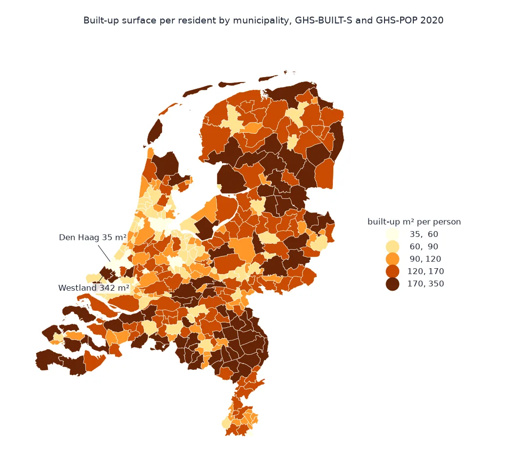
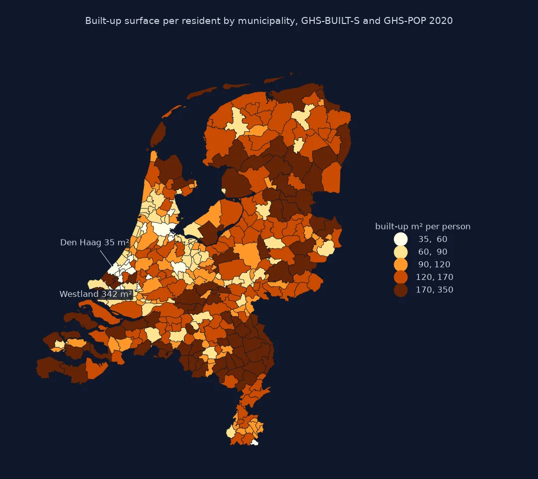
Den Haag, Amsterdam and Leiden have the least built-up surface per resident, 35 to 44 m². Westland, the greenhouse district between Den Haag and Rotterdam, has the most, 342 m², followed by two rural municipalities. Across all 355 municipalities, the denser the municipality, the less built-up area per person, with a rank correlation of -0.82.

Who built most per new resident

The data used on this page

GHS-BUILT-S and GHS-POP R2023A at 30 arc-seconds for the 1975, 2000 and 2020 epochs (tile R4_C19), and the 2020 country and municipality boundaries from the PDOK CBS gebiedsindelingen web feature service. The indicator follows the UN-Habitat metadata for SDG indicator 11.3.1.

import io
import zipfile
from pathlib import Path

import geopandas as gpd
import numpy as np
import rasterio
import requests
from exactextract import exact_extract
from rasterio.mask import mask

Path("data").mkdir(exist_ok=True)
GHSL = "https://jeodpp.jrc.ec.europa.eu/ftp/jrc-opendata/GHSL"
def tile(kind, year):
    name = f"GHS_{kind}_E{year}_GLOBE_R2023A_4326_30ss"
    tif = Path("data", f"{name}_V1_0_R4_C19.tif")
    if not tif.exists():
        url = f"{GHSL}/GHS_{kind}_GLOBE_R2023A/{name}/V1-0/tiles/{tif.stem}.zip"
        zipfile.ZipFile(io.BytesIO(requests.get(url, timeout=600).content)).extract(tif.name, "data")
    return tif
for layer in ("landsdeel", "gemeente"):
    path = Path("data", f"{layer}_2020.geojson")
    if not path.exists():
        path.write_bytes(requests.get("https://service.pdok.nl/cbs/gebiedsindelingen/2020/wfs/v1_0", timeout=300, params={
            "service": "WFS", "version": "2.0.0", "request": "GetFeature", "typeName": f"gebiedsindelingen:{layer}_gegeneraliseerd",
            "outputFormat": "application/json", "srsName": "EPSG:28992"}).content)
NL = gpd.read_file("data/landsdeel_2020.geojson").dissolve()
GM = gpd.read_file("data/gemeente_2020.geojson")
def clip(path, area):
    with rasterio.open(path) as src:
        a, _ = mask(src, area.to_crs(src.crs).geometry, crop=True, filled=False)
    return a[0].astype("float64")
for y in (1975, 2000, 2020):
    tile("BUILT_S", y); tile("POP", y)
print(f"{len(GM)} municipalities; land {NL.area.iloc[0] / 1e6:,.0f} km2")

355 municipalities; land 35,085 km2

The boundaries cover 35,085 km² of land in 355 municipalities.

Example 1: who built most per new resident

For each municipality, divide the built-up area added between 1975 and 2020 by the people added, for municipalities that grew by at least 5,000:

GM["added_m2"] = GM.built_s_2020 - GM.built_s_1975
GM["added_people"] = GM.pop_2020 - GM.pop_1975
grew = GM[GM.added_people >= 5_000].copy()
grew["m2_per_new"] = grew.added_m2 / grew.added_people
fmt = {"added_people": "{:,.0f}".format, "m2_per_new": "{:,.0f}".format}
print(f"{len(grew)} municipalities grew by 5,000+; median {grew.m2_per_new.median():,.0f} m2 of new built-up surface per new resident")
print(grew.nlargest(3, "m2_per_new")[["statnaam", "added_people", "m2_per_new"]].to_string(index=False, formatters=fmt))
print(grew.nsmallest(3, "m2_per_new")[["statnaam", "added_people", "m2_per_new"]].to_string(index=False, header=False, formatters=fmt))

204 municipalities grew by 5,000+; median 253 m2 of new built-up surface per new resident
    statnaam added_people m2_per_new
    Moerdijk        6,317        955
Het Hogeland        5,051        943
  Leeuwarden        6,113        871
Zoetermeer  85,096 39
   Haarlem  36,279 40
   Utrecht 173,584 44

Of the 204 municipalities that grew by 5,000 people or more, the median added 253 m² of built-up surface for each new resident. Moerdijk, with its industrial port, added 955 m² per new resident; Zoetermeer, Haarlem and Utrecht added about 40 m² per new resident, no more than the densest cities have per resident today.

Built-up per new resident.

What GHS-BUILT-S measures

Choropleth of Dutch municipalities by built-up square metres per resident in 2020, in five classes from 35 to 350: the large cities of the Randstad are lightest, Den Haag 35; rural municipalities in the north, east, Zeeland and Limburg are darkest, above 170, and Westland, the greenhouse district, is 342. — Built-up area per person.

GHS-BUILT-S measures built-up surface: the area covered by buildings and other roofed structures, detected from Sentinel-2 for recent epochs and from Landsat for the back-cast ones, in square metres per cell. It does not include roads, car parks or gardens, so it measures less land than "urban area" in land-cover products, and it does not separate homes from offices, warehouses and greenhouses. Built-up area per person therefore mixes housing space with everything else a society builds, which is why rural municipalities with farms, barns and glasshouses can have more of it per resident than cities.

The SDG 11.3.1 ratio compares two growth rates rather than two levels, so it asks whether new building outpaced new residents. A ratio above 1 means built-up area per person rose; below 1, it fell, as happens when growth is mostly densification. It is sensitive to the period, to how built-up area is defined, and, for small areas, to small absolute numbers: a municipality that gained few residents can show any ratio at all.

Same release, residential use and shrinking places

Built-up per person traps.

Same release for both layers: GHS-POP is distributed over GHS-BUILT volume in the same release, so the two are not independent; built-up area per person from them is internally consistent, not an independent measurement.
Residential only: R2023A also publishes a non-residential share (GHS-BUILT-C and the NRES variants of the built-up layers); use them for housing space per person.
Cell area: built-up square metres per cell are absolute, so sums need no cell-area correction, unlike densities on this grid.
Shrinking places: where population fell, the population growth rate is negative and the ratio changes sign; report the two rates separately there.

Internal links

How to map population change since 1975 with GHSL in Python — the population side of the epochs
How to classify degree of urbanisation with GHSL in Python — built-up and population combined into classes
How to measure urban growth from NLCD in Python — built-up growth from land cover

FAQ

How do I calculate built-up area per person with GHSL?

Sum GHS-BUILT-S and GHS-POP for the same epoch over the same area and divide; the built-up layer is already in square metres per cell.

What is SDG indicator 11.3.1?

The ratio of land consumption rate to population growth rate: the log growth rate of built-up area divided by the log growth rate of population over the same period.

Does GHS-BUILT-S include roads?

No; it measures built-up surface of buildings and other roofed structures, not roads or other sealed surfaces.

Why do rural areas have more built-up area per person?

Farms, barns, greenhouses and industrial buildings are built-up surface too, and there are fewer residents to divide them among.