Degree of Urbanisation Explained

Problem statement

Every country draws the line between urban and rural differently: by the size of a settlement, its administrative status, its density, or the share of people working outside farming. Comparing "urban population" across countries with those definitions compares definitions, not countries. The Degree of Urbanisation replaces them with one rule applied to a 1 km population grid everywhere, endorsed by the UN Statistical Commission in 2020 for international comparisons.

This page explains how the rule works by applying its first level directly to Statistics Netherlands' census grid, compares the result with the GHSL's ready-made GHS-SMOD classification and with the Dutch national urbanity classes, and tests how sensitive the result is to the thresholds.

Quick answer

The first level sorts 1 km cells into cities, towns and semi-dense areas, and rural areas, using two density thresholds and two population sizes. On the census grid:

centre = clusters(D >= 1_500, connectivity=4, min_pop=50_000)
cluster = clusters(D >= 300, connectivity=8, min_pop=5_000) & ~centre
share = {"cities": P[centre].sum(), "towns and semi-dense areas": P[cluster].sum(), "rural areas": P[~centre & ~cluster].sum()}
total = sum(share.values())
for k, v in share.items():
    print(f"{k:>27}: {v:>11,.0f}  {v / total:.1%}")

                     cities:   7,972,715  47.6%
 towns and semi-dense areas:   6,688,330  40.0%
                rural areas:   2,079,740  12.4%

Applied to the census grid, the first level puts 47.6% of the published residents in cities, 40.0% in towns and semi-dense areas, and 12.4% in rural areas.

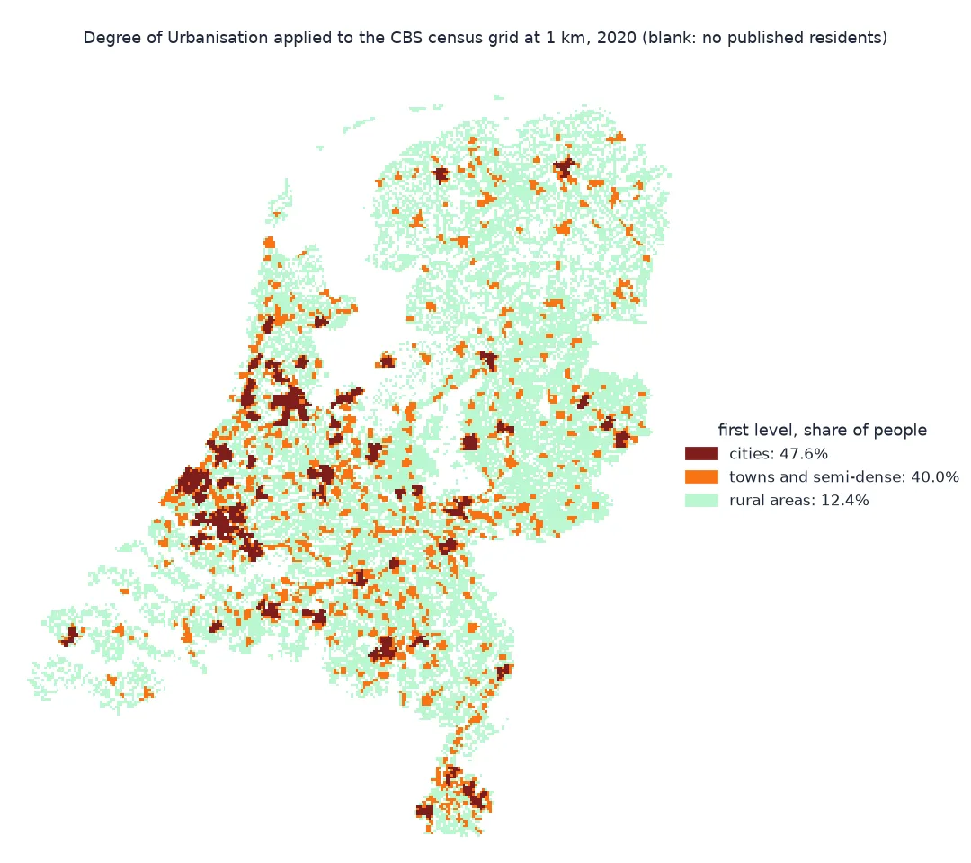
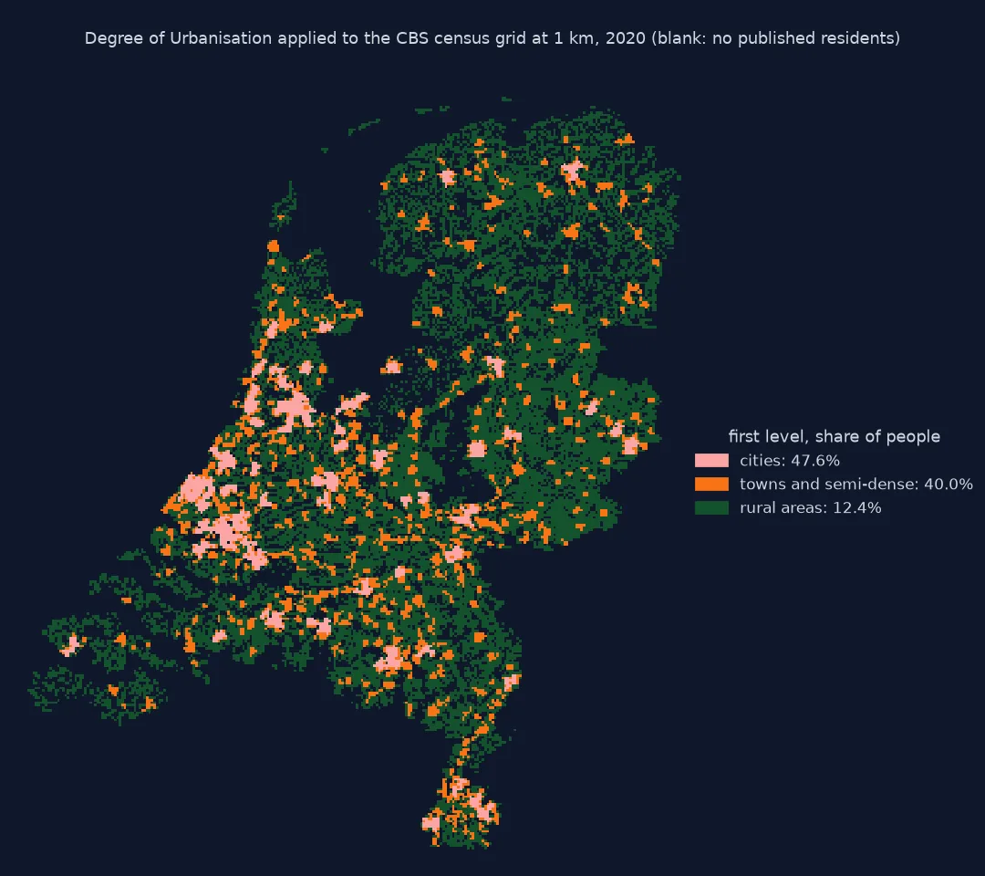
Two thresholds and two sizes, census against model, sensitivity

1. The two thresholds and two sizes

Density is people per km² of a 1 km cell; size is the population of a connected group of cells. Count how many cells pass each density threshold, and how many groups then reach the size:

for dens, conn, size in ((1_500, 4, 50_000), (300, 8, 5_000)):
    lab, n = ndimage.label(D >= dens, structure=STRUCT[conn])
    pops = ndimage.sum(P, lab, range(1, n + 1))
    print(f"cells >= {dens:,} per km2: {(D >= dens).sum():,}; groups ({conn}-connected): {n:,}; groups with {size:,}+ people: {(pops >= size).sum():,}")

cells >= 1,500 per km2: 3,457; groups (4-connected): 692; groups with 50,000+ people: 47
cells >= 300 per km2: 7,224; groups (8-connected): 1,117; groups with 5,000+ people: 300

3,457 cells reach 1,500 people per km², in 692 edge-connected groups, of which only 47 total 50,000 people and become urban centres. 7,224 cells reach 300 per km², in 1,117 groups; 300 of those total 5,000 and become urban clusters. Most dense groups are too small to count.

2. Census grid against GHS-SMOD

The GHSL applies the same rule to its modelled population grid, with a few refinements: smoothed edges of urban centres, gaps filled, and highly built-up cells admitted. Compare the shares:

print(f"{'':>27}  census grid   GHS-SMOD 2020")
for k in share:
    print(f"{k:>27}:      {share[k] / total:5.1%}          {SMOD[k]:5.1%}")

                             census grid   GHS-SMOD 2020
                     cities:      47.6%          49.0%
 towns and semi-dense areas:      40.0%          35.3%
                rural areas:      12.4%          15.7%

The two agree on the city share within 1.4 points, 47.6% against 49.0%. They differ more on the split between towns and rural areas: the census grid puts more people in towns, 40.0% against 35.3%, and fewer in rural areas. Two effects widen the gap in the same direction: the census grid leaves out the residents of its smallest squares, who are mostly rural, and the model, as the cell-by-cell comparison found, puts too many people in sparsely populated cells.

3. How sensitive the result is

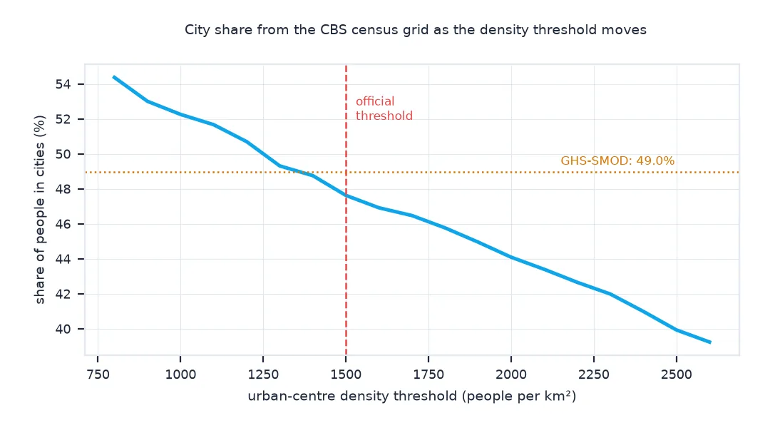
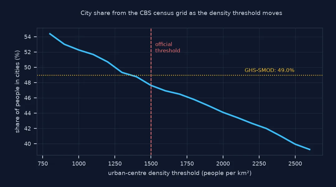
The thresholds are conventions. Move the urban-centre density threshold and see how much of the population changes class:

for dens in (1_000, 1_250, 1_500, 1_750, 2_000):
    c = clusters(D >= dens, connectivity=4, min_pop=50_000)
    print(f"urban-centre threshold {dens:>5,} per km2: cities hold {P[c].sum() / total:.1%} of people in {ndimage.label(c, structure=STRUCT[4])[1]} centres")

urban-centre threshold 1,000 per km2: cities hold 52.3% of people in 51 centres
urban-centre threshold 1,250 per km2: cities hold 49.7% of people in 48 centres
urban-centre threshold 1,500 per km2: cities hold 47.6% of people in 47 centres
urban-centre threshold 1,750 per km2: cities hold 46.3% of people in 48 centres
urban-centre threshold 2,000 per km2: cities hold 44.1% of people in 46 centres

Moving the threshold from 1,000 to 2,000 people per km² moves the city share from 52.3% to 44.1%, while the number of urban centres hardly changes, 46 to 51. The threshold mostly decides how far each centre's edge reaches, not how many centres there are.

The Dutch national urbanity classes

The data used on this page

The CBS 100 m grid, final 2020 edition, summed to 1 km cells of the Dutch RD New grid; GHS-SMOD R2023A version 2.0 and GHS-POP R2023A at 1 km for 2020 (tiles R3_C19 and R4_C19); the land boundary from the PDOK CBS gebiedsindelingen web feature service; and the population by urbanity class from StatLine table 70072ned.

import io
import json
import zipfile
from pathlib import Path

import geopandas as gpd
import numpy as np
import pyogrio
import rasterio
import requests
from rasterio.mask import mask
from rasterio.merge import merge
from scipy import ndimage

Path("data").mkdir(exist_ok=True)
GPKG = Path("data/cbs_vk100_2020_vol.gpkg")
if not GPKG.exists():
    url = "https://www.cbs.nl/-/media/cbs/dossiers/nederland-regionaal/vierkanten/100/2023-cbs_vk100_2020_vol.zip"
    zipfile.ZipFile(io.BytesIO(requests.get(url, timeout=900).content)).extract(GPKG.name, "data")
V = pyogrio.read_dataframe(GPKG, columns=["crs28992res100m", "aantal_inwoners"], read_geometry=False)
V = V[V.aantal_inwoners > 0]
xy = V.crs28992res100m.str.extract(r"E(\d+)N(\d+)").astype(int).to_numpy() // 10           # 1 km cell index
x0, y0 = xy.min(axis=0)
P = np.zeros((xy[:, 1].max() - y0 + 1, xy[:, 0].max() - x0 + 1))
np.add.at(P, (xy[:, 1] - y0, xy[:, 0] - x0), V.aantal_inwoners.to_numpy(float))
D = P / 1.0                                                                                 # people per km2 of a 1 km cell
STRUCT = {4: ndimage.generate_binary_structure(2, 1), 8: ndimage.generate_binary_structure(2, 2)}
def clusters(cells, connectivity, min_pop):
    """Cells belonging to connected groups of `cells` whose population reaches min_pop."""
    lab, n = ndimage.label(cells, structure=STRUCT[connectivity])
    pops = ndimage.sum(P, lab, range(1, n + 1))
    keep = np.r_[False, pops >= min_pop]
    return keep[lab]
GHSL = "https://jeodpp.jrc.ec.europa.eu/ftp/jrc-opendata/GHSL"
def tiles(kind, v):
    out = []
    for t in ("R3_C19", "R4_C19"):
        name = f"GHS_{kind}_E2020_GLOBE_R2023A_54009_1000"
        tif = Path("data", f"{name}_{v}_{t}.tif")
        if not tif.exists():
            url = f"{GHSL}/GHS_{kind}_GLOBE_R2023A/{name}/{v.replace('_', '-')}/tiles/{tif.stem}.zip"
            zipfile.ZipFile(io.BytesIO(requests.get(url, timeout=600).content)).extract(tif.name, "data")
        out.append(rasterio.open(tif))
    return out
B = Path("data/landsdeel_2020.geojson")
if not B.exists():
    B.write_bytes(requests.get("https://service.pdok.nl/cbs/gebiedsindelingen/2020/wfs/v1_0", timeout=300, params={
        "service": "WFS", "version": "2.0.0", "request": "GetFeature", "typeName": "gebiedsindelingen:landsdeel_gegeneraliseerd",
        "outputFormat": "application/json", "srsName": "EPSG:28992"}).content)
NL = gpd.read_file(B).dissolve().to_crs("ESRI:54009")
def clipped(srcs):
    a, tf = merge(srcs)
    with rasterio.MemoryFile() as mf:
        with mf.open(driver="GTiff", height=a.shape[1], width=a.shape[2], count=1, dtype=a.dtype, crs="ESRI:54009", transform=tf) as ds:
            ds.write(a)
            out, _ = mask(ds, NL.geometry, crop=True, filled=False)
    return out[0]
smod, spop = clipped(tiles("SMOD", "V2_0")), clipped(tiles("POP", "V1_0"))
k = ~smod.mask & ~spop.mask & (spop.data > 0)
by = {d: spop.data[k & (smod.data // 10 == d)].sum() for d in (3, 2, 1)}
SMOD = {"cities": by[3] / sum(by.values()), "towns and semi-dense areas": by[2] / sum(by.values()), "rural areas": by[1] / sum(by.values())}
U = Path("data/cbs_urbanity_2020.json")
if not U.exists():
    U.write_bytes(requests.get("https://opendata.cbs.nl/ODataApi/odata/70072ned/TypedDataSet", timeout=300, params={
        "$filter": "Perioden eq '2020JJ00' and substring(RegioS,0,2) eq 'NL'",
        "$select": "RegioS,TotaleBevolking_1,ZeerSterkStedelijk_22,SterkStedelijk_23,MatigStedelijk_24,WeinigStedelijk_25,NietStedelijk_26"}).content)
URB = json.loads(U.read_text())["value"][0]
print(f"census grid: {P.shape[1]} x {P.shape[0]} cells of 1 km, {P.sum():,.0f} people; GHS-SMOD cells with population: {k.sum():,}")

census grid: 265 x 305 cells of 1 km, 16,740,785 people; GHS-SMOD cells with population: 33,401

The census squares make a grid of 265 by 305 cells of 1 km holding 16,740,785 published residents; GHS-SMOD has 33,401 populated cells inside the country.

Example 1: the Dutch national urbanity classes

Statistics Netherlands classifies every neighbourhood by the density of addresses around it, from "very strongly urban" at 2,500 or more addresses per km² to "not urban" below 500. Put its five classes beside the three degrees:

classes = {"very strongly urban": "ZeerSterkStedelijk_22", "strongly urban": "SterkStedelijk_23", "moderately urban": "MatigStedelijk_24",
           "hardly urban": "WeinigStedelijk_25", "not urban": "NietStedelijk_26"}
for name, key in classes.items():
    print(f"{name:>20}: {URB[key] / URB['TotaleBevolking_1']:.1%}")
print(f"top two classes together: {(URB['ZeerSterkStedelijk_22'] + URB['SterkStedelijk_23']) / URB['TotaleBevolking_1']:.1%}; "
      f"cities by the census-grid rule: {share['cities'] / total:.1%}")

 very strongly urban: 24.0%
      strongly urban: 25.1%
    moderately urban: 17.1%
        hardly urban: 17.0%
           not urban: 16.9%
top two classes together: 49.0%; cities by the census-grid rule: 47.6%

The national classes are built differently, on the density of addresses around each neighbourhood rather than on 1 km cells, and have five levels. Even so, the two most urban classes together hold 49.0% of the population, close to the city share by the census-grid rule, 47.6%, and the least urban class 16.9%, close to GHS-SMOD's rural 15.7%. The agreement is useful but should not be read as equivalence: the classes are drawn around different units with different thresholds.

Density combined with size

The Degree of Urbanisation works on a regular grid so that a cell means the same everywhere, and it combines density with size so that a dense village does not count as a city. At the first level, an urban centre is a group of contiguous 1 km cells, connected by their edges, each with at least 1,500 inhabitants, totalling at least 50,000. An urban cluster is a group of cells with at least 300 inhabitants each, connected also at corners, totalling at least 5,000. Cells in urban centres are cities; other cells in urban clusters are towns and semi-dense areas; the rest are rural. Local administrative units are then classified by where most of their population lives, which is how the method produces national statistics.

Because the rule is fixed, differences between countries are differences between countries. Its limits follow from the same fixedness. The 1 km grid and its origin decide which cells cross a threshold; the thresholds are conventions chosen to work in many settlement systems, not natural breaks; and the input grid matters, as the census and modelled versions on this page show. For international comparison those are acceptable costs; for planning inside one country, national classes built on local data usually say more.

The second level and permanent land

• The second level: the full method splits towns and semi-dense areas into dense and semi-dense clusters and suburban cells, and rural areas into villages, dispersed and mostly uninhabited cells; GHS-SMOD publishes all seven classes.
• Simplified here: the census-grid version on this page applies the first-level thresholds without the smoothing, gap filling and built-up criterion GHS-SMOD adds, which is part of why the two differ.
• Grid alignment: the census grid here is on the RD New kilometre grid, GHS-SMOD on Mollweide; shifting a grid by half a cell can move a town across a threshold.
• Permanent land: the official method measures density per km² of permanent land, so coastal and lakeside cells are not penalised for water; the simple version here divides by the whole cell.

Internal links

• How to classify degree of urbanisation with GHSL in Python — using GHS-SMOD
• How to delineate an urban extent from GHSL in Python — urban centres built by hand
• Population grids explained — the census and modelled grids used here

FAQ

What is the Degree of Urbanisation?

A method endorsed by the UN Statistical Commission in 2020 that classifies 1 km grid cells, and then areas, into cities, towns and semi-dense areas, and rural areas, using population density and the size of connected groups of cells.

What are the thresholds in the Degree of Urbanisation?

Urban centres: cells of at least 1,500 inhabitants per km² in edge-connected groups of at least 50,000 people. Urban clusters: cells of at least 300 per km² in groups of at least 5,000.

Why does GHS-SMOD differ from my own classification?

It uses a modelled population grid, smooths and fills the urban centres, admits highly built-up cells, and measures density on permanent land; a census-based version with the bare thresholds will differ by a few points.

How does the Degree of Urbanisation compare with national definitions?

It is designed to be comparable between countries, not to match any one national definition; in the Netherlands its city share happens to be close to the share in CBS's two most urban classes.