
How to Classify Degree of Urbanisation with GHSL in Python
On this page
Problem statement
"Urban" means something different in every country's statistics, which makes international comparisons of urban population meaningless. The Degree of Urbanisation, endorsed by the UN Statistical Commission in 2020, fixes that with one rule applied to 1 km population grid cells everywhere: cities are dense, populous clusters of cells, towns and suburbs are smaller or looser ones, and the rest is rural. The GHSL publishes the classification ready-made as GHS-SMOD, for every epoch from 1975 to 2030.
This page reads GHS-SMOD and GHS-POP for the Netherlands at 1 km, merges the two tiles the country straddles, counts population by settlement class and by the three degrees, extracts the urban centres as named clusters, and compares 1975 with 2020.
Quick answer
Merge the tiles, mask with the boundary in the grid's CRS, and sum population by SMOD class:
smod, tf = clip(merged("SMOD", 2020))
pop, _ = clip(merged("POP", 2020))
ok = ~smod.mask & ~pop.mask
by_class = pd.Series(pop.data[ok]).groupby(smod.data[ok]).sum()
share = (by_class / by_class.sum()).rename(index=CLASSES)
print(f"population on {ok.sum():,} 1 km cells: {by_class.sum():,.0f}")
print(share.sort_values(ascending=False).map("{:.1%}".format).to_string())
population on 35,012 1 km cells: 17,369,596
urban centre 49.0%
dense urban cluster 20.4%
suburban or peri-urban 12.8%
low density rural 9.6%
rural cluster 4.7%
semi-dense urban cluster 2.2%
very low density rural 1.4%
water 0.0%
The 35,012 cells hold 17,369,596 people. Almost half, 49.0%, live in urban centres and another fifth in dense urban clusters; the very low density rural cells, the most common class by area, hold 1.4%.
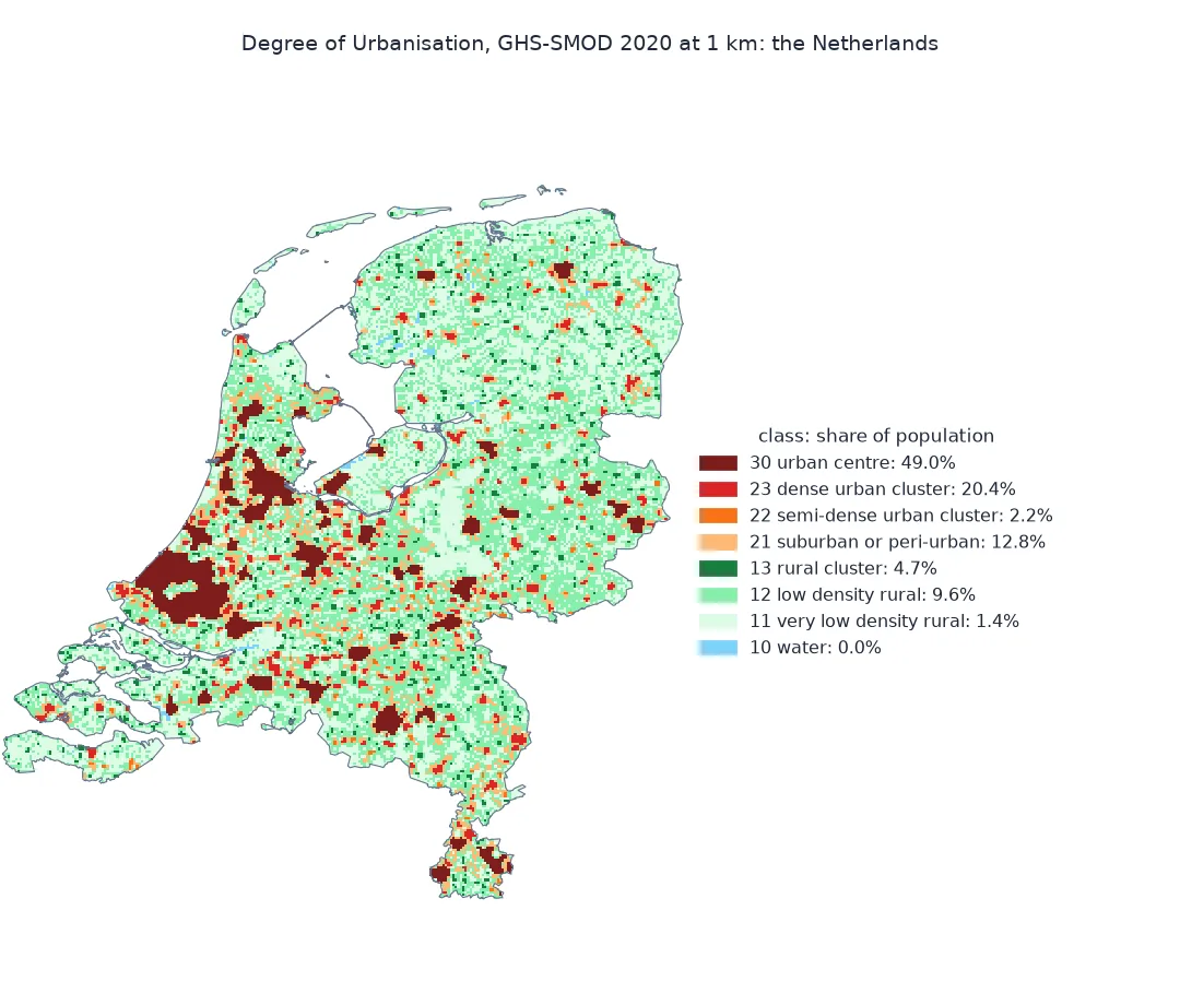
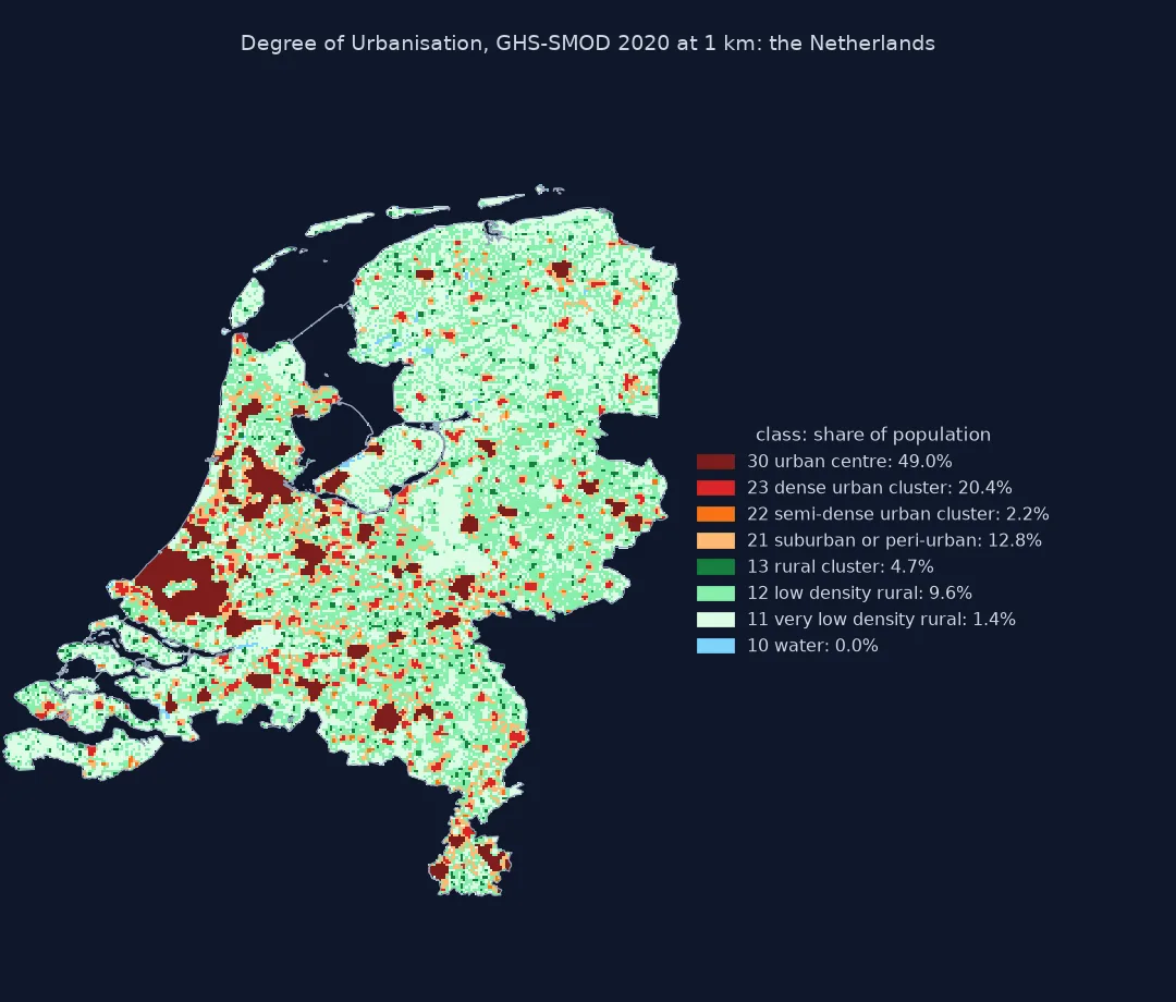
Read the classes, collapse to three degrees, cluster centres
1. Read the classes
SMOD stores a two-digit code per cell: the first digit is the degree (3 city, 2 town or suburb, 1 rural), the second the settlement type within it:
cells = pd.Series(smod.data[ok]).value_counts().sort_index()
for code, n in cells.items():
    print(f"{code}  {CLASSES[code]:<28} {n:>6,} cells")
with rasterio.open(merged("SMOD", 2020)) as src:
    print(f"grid: {src.res[0]:.0f} m cells, {src.crs.to_string()[:30]}..., nodata {src.nodata}")
10 water 153 cells
11 very low density rural 12,855 cells
12 low density rural 13,619 cells
13 rural cluster 1,116 cells
21 suburban or peri-urban 3,135 cells
22 semi-dense urban cluster 224 cells
23 dense urban cluster 1,382 cells
30 urban centre 2,528 cells
grid: 1000 m cells, ESRI:54009..., nodata -200.0
Low and very low density rural cells cover 26,474 of the 35,012 km²; urban centres cover 2,528. The grid is 1 km in World Mollweide (ESRI:54009) with -200 as nodata.
2. Collapse to the three degrees
The first level of the classification has three classes, which is what the international statistics report:
degree = {3: "cities", 2: "towns and semi-dense areas", 1: "rural areas"}
d = by_class.groupby(by_class.index // 10).sum()
d.index = d.index.map(degree)
area = cells.groupby(cells.index // 10).sum()
area.index = area.index.map(degree)
print(pd.DataFrame({"population": d.round(), "share": (d / d.sum()).map("{:.1%}".format), "km2": area}).to_string())
population share km2
rural areas 2727094.0 15.7% 27743
towns and semi-dense areas 6135948.0 35.3% 4741
cities 8506554.0 49.0% 2528
At the first level, 49.0% of the population lives in cities, 35.3% in towns and semi-dense areas, and 15.7% in rural areas, which take 79% of the land, 27,743 km².
3. Urban centres as clusters
An urban centre is a contiguous group of class 30 cells. Label the groups with scipy.ndimage.label, sum each one's population, and name each after the municipalities that hold most of its people:
lab, n = ndimage.label(smod.filled(0) == 30)
pc = pd.Series(ndimage.sum(pop.filled(0), lab, range(1, n + 1)), index=range(1, n + 1))
print(f"{n} urban centres holding {pc.sum():,.0f} people")
r, c = np.nonzero(lab)
xs, ys = rasterio.transform.xy(tf, r, c)
cells_ = gpd.GeoDataFrame({"centre": lab[r, c], "people": pop.filled(0)[r, c]}, geometry=gpd.points_from_xy(xs, ys), crs=MOLL)
cells_ = cells_.to_crs(28992).sjoin(GM[["statnaam", "geometry"]])
for k, people in pc.nlargest(6).items():
    own = cells_[cells_.centre == k].groupby("statnaam").people.sum().nlargest(2)
    print(f"{' + '.join(own.index):<26} {people:>10,.0f} people, {(lab == k).sum():>3} km2, {cells_[cells_.centre == k].statnaam.nunique():>2} municipalities")
45 urban centres holding 8,506,554 people
Rotterdam + 's-Gravenhage 2,116,766 people, 668 km2, 21 municipalities
Amsterdam + Zaanstad 1,171,569 people, 288 km2, 11 municipalities
Utrecht + Nieuwegein 493,888 people, 115 km2, 6 municipalities
Eindhoven + Veldhoven 284,160 people, 96 km2, 4 municipalities
Leiden + Katwijk 266,405 people, 67 km2, 9 municipalities
Dordrecht + Zwijndrecht 252,804 people, 86 km2, 8 municipalities
The classification finds 45 urban centres holding 8,506,554 people. The largest joins Rotterdam and Den Haag with 19 other municipalities into one centre of 2.1 million on 668 km², because the 1 km cells between them are dense enough to connect; the hand-built centres in the urban extent guide keep the two apart. Amsterdam and Zaanstad form the second, with 1.2 million.
The Netherlands in 1975 against 2020
The data used on this page
GHS-SMOD R2023A, version 2.0, and GHS-POP R2023A, both at 1 km in World Mollweide for 1975 and 2020 (tiles R3_C19 and R4_C19), and the 2020 country and municipality boundaries from the PDOK CBS gebiedsindelingen web feature service.
import io
import zipfile
from pathlib import Path

import geopandas as gpd
import numpy as np
import pandas as pd
import rasterio
import requests
from rasterio.mask import mask
from rasterio.merge import merge
from scipy import ndimage

Path("data").mkdir(exist_ok=True)
GHSL = "https://jeodpp.jrc.ec.europa.eu/ftp/jrc-opendata/GHSL"
MOLL = "ESRI:54009"
CLASSES = {30: "urban centre", 23: "dense urban cluster", 22: "semi-dense urban cluster", 21: "suburban or peri-urban",
           13: "rural cluster", 12: "low density rural", 11: "very low density rural", 10: "water"}
def tile(kind, year, t):
    v = "V2_0" if kind == "SMOD" else "V1_0"
    name = f"GHS_{kind}_E{year}_GLOBE_R2023A_54009_1000"
    tif = Path("data", f"{name}_{v}_{t}.tif")
    if not tif.exists():
        url = f"{GHSL}/GHS_{kind}_GLOBE_R2023A/{name}/{v.replace('_', '-')}/tiles/{tif.stem}.zip"
        zipfile.ZipFile(io.BytesIO(requests.get(url, timeout=600).content)).extract(tif.name, "data")
    return tif
def merged(kind, year):
    out = Path("data", f"{kind}_{year}_nl_1km.tif")
    if not out.exists():
        srcs = [rasterio.open(tile(kind, year, t)) for t in ("R3_C19", "R4_C19")]
        a, transform = merge(srcs)
        profile = srcs[0].profile | {"height": a.shape[1], "width": a.shape[2], "transform": transform}
        with rasterio.open(out, "w", **profile) as dst:
            dst.write(a)
    return out
B = Path("data/landsdeel_2020.geojson")
G = Path("data/gemeente_2020.geojson")
for path, layer in ((B, "landsdeel"), (G, "gemeente")):
    if not path.exists():
        path.write_bytes(requests.get("https://service.pdok.nl/cbs/gebiedsindelingen/2020/wfs/v1_0", timeout=300, params={
            "service": "WFS", "version": "2.0.0", "request": "GetFeature", "typeName": f"gebiedsindelingen:{layer}_gegeneraliseerd",
            "outputFormat": "application/json", "srsName": "EPSG:28992"}).content)
NL, GM = gpd.read_file(B).dissolve(), gpd.read_file(G)
def clip(path):
    with rasterio.open(path) as src:
        a, transform = mask(src, NL.to_crs(src.crs).geometry, crop=True, filled=False)
    return a[0], transform
print({kind: rasterio.open(merged(kind, 2020)).shape for kind in ("SMOD", "POP")})
{'SMOD': (2000, 1000), 'POP': (2000, 1000)}
Each merged layer is 2,000 by 1,000 cells, the two 1,000 km tiles stacked.
Example 1: 1975 against 2020
The same rule applied to the 1975 epoch shows how the country's settlement pattern moved:
def degrees(year):
    s, _ = clip(merged("SMOD", year)); p, _ = clip(merged("POP", year))
    k = ~s.mask & ~p.mask
    return pd.Series(p.data[k]).groupby(s.data[k] // 10).sum().rename(index=degree)
D = pd.DataFrame({y: degrees(y) for y in (1975, 2020)})
D["change"] = D[2020] - D[1975]
print(D.round(-3).astype(int).to_string(formatters={c: "{:,}".format for c in D.columns}))
print((D[[1975, 2020]] / D[[1975, 2020]].sum()).map("{:.1%}".format).to_string())
1975 2020 change
rural areas 2,501,000 2,727,000 226,000
towns and semi-dense areas 5,560,000 6,136,000 576,000
cities 5,559,000 8,507,000 2,948,000
1975 2020
rural areas 18.4% 15.7%
towns and semi-dense areas 40.8% 35.3%
cities 40.8% 49.0%
Cities gained 2,948,000 people between 1975 and 2020, towns and semi-dense areas 576,000 and rural areas 226,000. The city share rose from 40.8% to 49.0%, a mix of growth inside 1975's cities and cells that crossed the thresholds into the city class, which a table by class cannot separate; comparing the two SMOD layers cell by cell can.
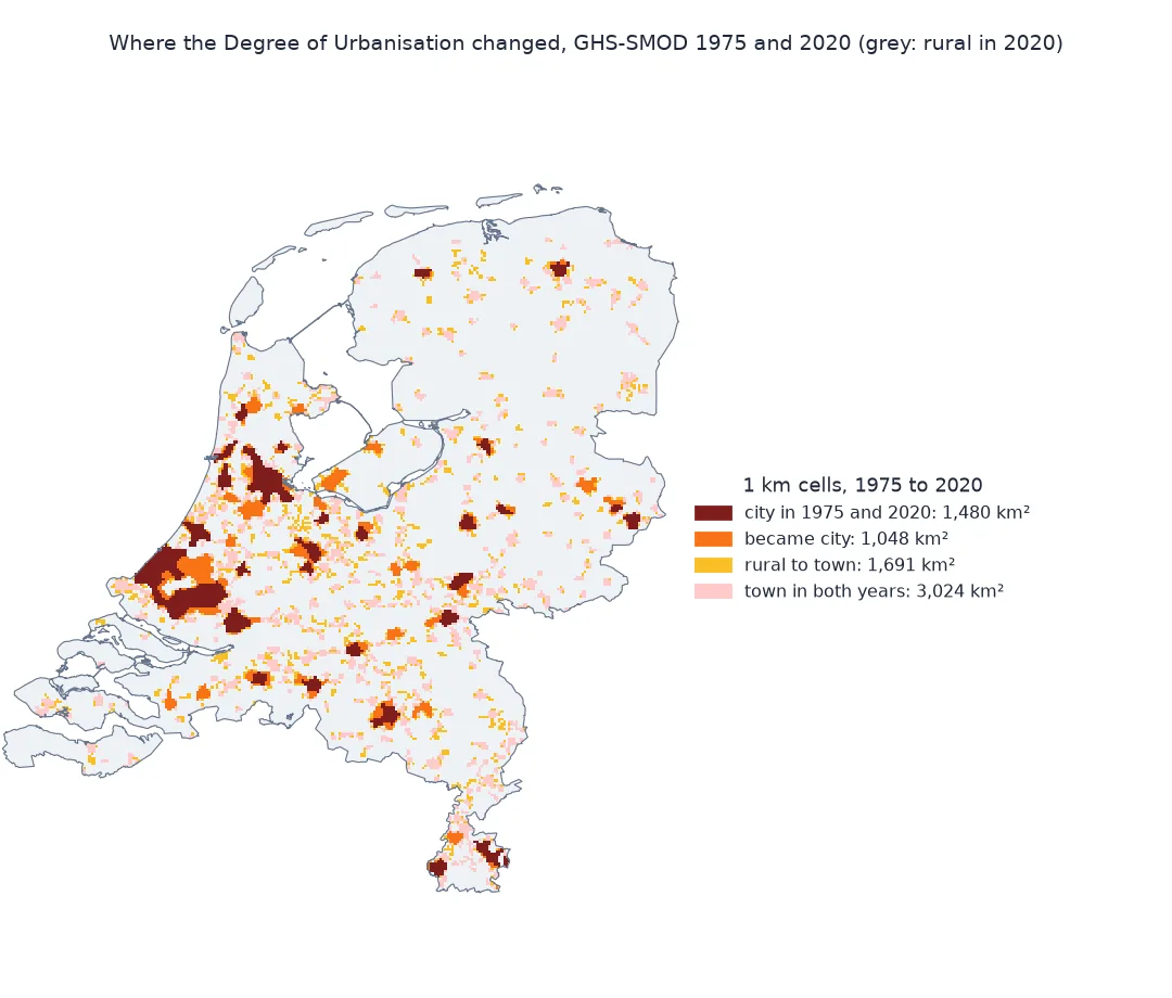
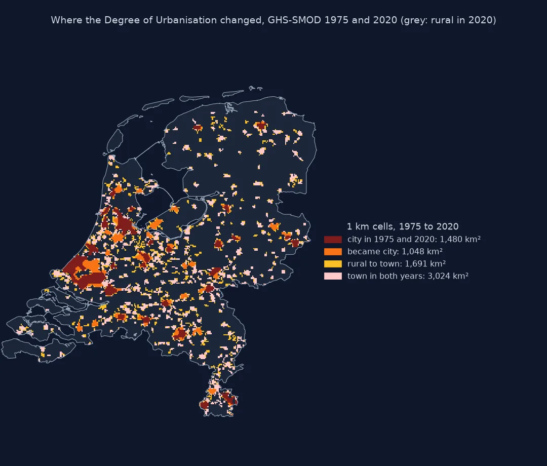
Density per land area and cluster thresholds
The classification works on 1 km cells, with densities measured per km² of permanent land. An urban centre is a cluster of cells with at least 1,500 inhabitants per km² totalling at least 50,000 people, its edge smoothed and holes under 15 km² filled; GHSL also admits cells with a high built-up density, so that office parks and malls do not split a city. A dense urban cluster meets the same density with 5,000 to 50,000 people. Urban clusters at the first level are contiguous cells of at least 300 per km² totalling 5,000; within them, semi-dense clusters need 900 per km² and 2,500 people at least 2 km from a denser cluster, and the rest are suburban or peri-urban. Outside urban clusters, rural clusters have 300 per km² and 500 to 5,000 people, and the remaining cells are low density rural (50 or more per km²) or very low density rural.
Because the thresholds are fixed and the grid is the same everywhere, the classes mean the same thing in the Netherlands as in Nigeria, which national definitions do not. The cost is that the classes depend on the population grid's errors and on where its cell edges fall; a town split by a cell edge can drop below a threshold. For local planning, national definitions and finer grids remain better; for comparing countries or years, this is the standard.
Versions, Mollweide and two tiles
- Version: GHS-SMOD R2023A exists as V1-0 and V2-0; the JRC marks V1-0 obsolete, so use V2-0 and say so.
- Mollweide only at 1 km: SMOD is published in Mollweide; reproject vector data to
ESRI:54009rather than warping the classes, which are categorical and must not be resampled bilinearly. - Two tiles: the Netherlands crosses the boundary between tile rows R3 and R4; merge before masking, or half the country is missing.
- Degree of Urbanisation for areas: the method also classifies local administrative units by where their population lives; the GHSL publishes that separately.
Internal links
- How to delineate an urban extent from GHSL in Python — building urban centres by hand
- How to download and clip the GHSL population grid in Python — the population layer
- How to map population change since 1975 with GHSL in Python — epochs over time
FAQ
What is GHS-SMOD?
The GHSL settlement model layer: the Degree of Urbanisation classes for every 1 km cell of the globe, for each epoch from 1975 to 2030, computed from GHS-POP and GHS-BUILT.
What do the SMOD codes mean?
The first digit is the degree, 3 city, 2 town or semi-dense area, 1 rural; the second is the type, from 30 urban centre to 11 very low density rural, with 10 for water.
What share of the Dutch population lives in cities?
In GHS-SMOD and GHS-POP 2020, 49.0% of the Dutch population lives in the 45 urban centres, and 15.7% in rural areas.
Can I resample SMOD to another grid?
Only with nearest-neighbour or a mode filter; the values are codes, not quantities.