
How to Compute Population-Weighted Density in Python
On this page
Problem statement
The density of a municipality, its population over its area, mixes the people with every park, harbour, airport and field inside its boundary. Two cities with the same housing can get very different densities because one boundary includes farmland. Population-weighted density asks a different question: at what density does the average resident live? It averages the density of small cells, weighted by the people in them, so empty land inside the boundary stops mattering.
This page computes population-weighted density for Dutch municipalities from Statistics Netherlands' 100 m census squares, compares it with plain density, shows how it depends on the cell size, and repeats it with GHS-POP at 1 km.
Quick answer
Each square's density is its people over its area; weight those densities by the people:
def pwd(people, cell_km2):
    d = people / cell_km2
    return (people * d).sum() / people.sum()
ams = SQ[SQ.statnaam == "Amsterdam"].residents
print(f"Amsterdam: {ams.sum():,} residents in {len(ams):,} squares of 100 m")
print(f"plain density {OFF['GM0363'] / GM.set_index('statcode').km2['GM0363']:,.0f} per km2; population-weighted density {pwd(ams, 0.01):,.0f} per km2")
Amsterdam: 865,890 residents in 6,755 squares of 100 m
plain density 4,440 per km2; population-weighted density 20,249 per km2
Amsterdam's 865,890 residents in published squares live in 6,755 squares of 100 m. Its plain density is 4,440 per km² of land; the density at which its average resident lives is 20,249 per km², 4.6 times as high.
Plain and weighted density, cell-size dependence, rankings
1. Plain and weighted density for the largest municipalities
Compute both for the ten municipalities with the most people:
G = GM.set_index("statcode")
big = G.nlargest(10, "people")
T = pd.DataFrame({"municipality": big.statnaam,
                  "plain": big.people / big.km2,
                  "weighted_100m": [pwd(SQ[SQ.statcode == c].residents, 0.01) for c in big.index]})
T["ratio"] = T.weighted_100m / T.plain
print(T.sort_values("weighted_100m", ascending=False).to_string(index=False, formatters={
      "plain": "{:,.0f}".format, "weighted_100m": "{:,.0f}".format, "ratio": "{:.1f}x".format}))
municipality plain weighted_100m ratio
Amsterdam 4,440 20,249 4.6x
's-Gravenhage 6,378 16,729 2.6x
Rotterdam 2,212 16,465 7.4x
Utrecht 3,604 14,274 4.0x
Groningen 1,177 10,731 9.1x
Nijmegen 3,083 10,040 3.3x
Tilburg 1,861 9,491 5.1x
Eindhoven 2,634 9,144 3.5x
Almere 1,521 9,082 6.0x
Breda 1,432 8,259 5.8x
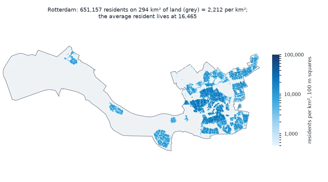
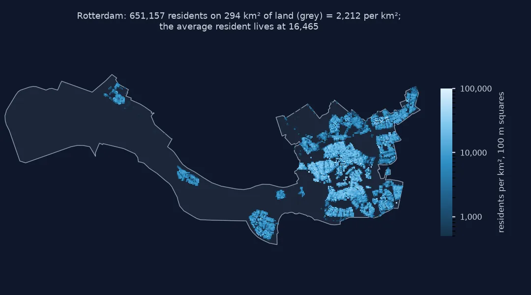
By plain density Den Haag is the densest of the ten by far and Groningen the sparsest. Weighted by population, Amsterdam comes first, and Rotterdam, which plain density puts sixth with 2,212 per km² because its municipality includes the port, moves up to third with 16,465. Groningen's ratio is the largest, 9.1: a compact city in a municipality with a lot of farmland.
2. It depends on the cell size
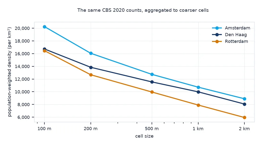
Aggregate the squares to 500 m and 1 km and recompute. Coarser cells average dense blocks with their surroundings:
for size in (1, 5, 10):
    agg = SQ.assign(kx=SQ.x // size, ky=SQ.y // size).groupby(["statcode", "kx", "ky"]).residents.sum()
    v = [pwd(agg[c], (size / 10) ** 2) for c in ("GM0363", "GM0518", "GM0599")]
    print(f"{size * 100:>5} m cells: Amsterdam {v[0]:>7,.0f}, Den Haag {v[1]:>7,.0f}, Rotterdam {v[2]:>7,.0f} per km2")
100 m cells: Amsterdam 20,249, Den Haag 16,729, Rotterdam 16,465 per km2
500 m cells: Amsterdam 12,734, Den Haag 11,544, Rotterdam 9,959 per km2
1000 m cells: Amsterdam 10,722, Den Haag 9,984, Rotterdam 7,911 per km2
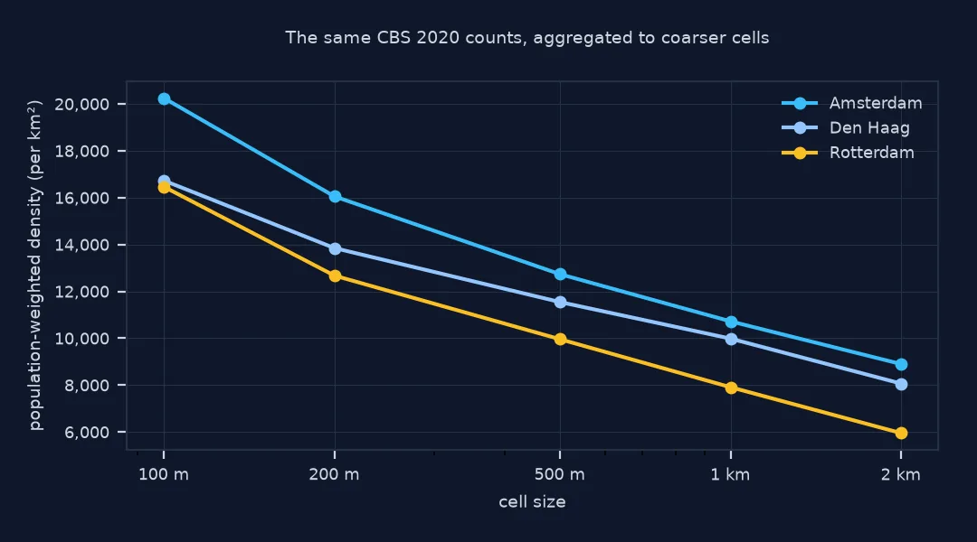
Going from 100 m to 1 km cells halves the weighted density of all three cities, from 20,249 to 10,722 in Amsterdam, and widens the gap between Den Haag and Rotterdam. The cell size is part of the measure.
3. Does the ranking change?
For all municipalities over 50,000 residents, compare the order by plain density with the order by weighted density:
M = G[G.people > 50_000].copy()
M["plain"] = M.people / M.km2
M["weighted"] = [pwd(SQ[SQ.statcode == c].residents, 0.01) for c in M.index]
rho = M.plain.rank().corr(M.weighted.rank())
M["moved"] = M.plain.rank(ascending=False) - M.weighted.rank(ascending=False)
print(f"{len(M)} municipalities; rank correlation {rho:.2f}")
print(M.reindex(M.moved.abs().sort_values(ascending=False).index).head(4)[["statnaam", "plain", "weighted", "moved"]].to_string(
      index=False, formatters={"plain": "{:,.0f}".format, "weighted": "{:,.0f}".format, "moved": "{:+.0f} places".format}))
88 municipalities; rank correlation 0.87
statnaam plain weighted moved
Hoorn 3,494 7,864 -33 places
Heerlen 1,912 7,197 -31 places
Sittard-Geleen 1,147 5,765 -31 places
Groningen 1,177 10,731 +27 places
Across the 88 municipalities over 50,000 residents the two orders agree broadly, with a rank correlation of 0.87, but some move a long way. Hoorn falls 33 places and Heerlen and Sittard-Geleen 31: their boundaries hold little empty land, so plain density flatters them, while their residents live at moderate densities. Groningen rises 27 places.
The same measure from GHS-POP
The data used on this page
The CBS 100 m grid, final 2020 edition, GHS-POP R2023A epoch 2020 at 1 km in Mollweide (tiles R3_C19 and R4_C19), the 2020 municipality boundaries from the PDOK CBS gebiedsindelingen web feature service, and each municipality's population on 1 January 2020 from StatLine table 03759ned.
import io
import json
import zipfile
from pathlib import Path

import geopandas as gpd
import numpy as np
import pandas as pd
import pyogrio
import rasterio
import requests
from rasterio.merge import merge

Path("data").mkdir(exist_ok=True)
GPKG = Path("data/cbs_vk100_2020_vol.gpkg")
if not GPKG.exists():
    url = "https://www.cbs.nl/-/media/cbs/dossiers/nederland-regionaal/vierkanten/100/2023-cbs_vk100_2020_vol.zip"
    zipfile.ZipFile(io.BytesIO(requests.get(url, timeout=900).content)).extract(GPKG.name, "data")
B = Path("data/gemeente_2020.geojson")
if not B.exists():
    B.write_bytes(requests.get("https://service.pdok.nl/cbs/gebiedsindelingen/2020/wfs/v1_0", timeout=300, params={
        "service": "WFS", "version": "2.0.0", "request": "GetFeature", "typeName": "gebiedsindelingen:gemeente_gegeneraliseerd",
        "outputFormat": "application/json", "srsName": "EPSG:28992"}).content)
C = Path("data/cbs_pop_2020.json")
if not C.exists():
    C.write_bytes(requests.get("https://opendata.cbs.nl/ODataApi/odata/03759ned/TypedDataSet", timeout=300, params={
        "$filter": "Geslacht eq 'T001038' and Leeftijd eq '10000' and BurgerlijkeStaat eq 'T001019' and Perioden eq '2020JJ00' "
                   "and (substring(RegioS,0,2) eq 'GM' or substring(RegioS,0,2) eq 'NL')",
        "$select": "RegioS,BevolkingOp1Januari_1"}).content)
OFF = {r["RegioS"].strip(): r["BevolkingOp1Januari_1"] for r in json.loads(C.read_text())["value"] if r["BevolkingOp1Januari_1"]}
GM = gpd.read_file(B)
GM["people"], GM["km2"] = GM.statcode.map(OFF), GM.area / 1e6
V = pyogrio.read_dataframe(GPKG, columns=["crs28992res100m", "aantal_inwoners"], read_geometry=False)
V = V[V.aantal_inwoners > 0]                                                       # published resident counts only
xy = V.crs28992res100m.str.extract(r"E(\d+)N(\d+)").astype(int)
pts = gpd.GeoDataFrame({"residents": V.aantal_inwoners.to_numpy(), "x": xy[0].to_numpy(), "y": xy[1].to_numpy()},
                       geometry=gpd.points_from_xy(xy[0] * 100 + 50, xy[1] * 100 + 50), crs=28992)
SQ = pts.sjoin(GM[["statcode", "statnaam", "geometry"]], predicate="within")
GHSL = "https://jeodpp.jrc.ec.europa.eu/ftp/jrc-opendata/GHSL/GHS_POP_GLOBE_R2023A"
tiles = []
for t in ("R3_C19", "R4_C19"):
    tif = Path("data", f"GHS_POP_E2020_GLOBE_R2023A_54009_1000_V1_0_{t}.tif")
    if not tif.exists():
        url = f"{GHSL}/GHS_POP_E2020_GLOBE_R2023A_54009_1000/V1-0/tiles/{tif.stem}.zip"
        zipfile.ZipFile(io.BytesIO(requests.get(url, timeout=600).content)).extract(tif.name, "data")
    tiles.append(rasterio.open(tif))
GHS, GHS_TF = merge(tiles)
print(f"{len(SQ):,} populated squares joined to {SQ.statcode.nunique()} municipalities; GHS-POP mosaic {GHS.shape[2]} x {GHS.shape[1]} km")
379,704 populated squares joined to 355 municipalities; GHS-POP mosaic 1000 x 2000 km
379,704 squares with a published resident count are joined to all 355 municipalities; the GHS-POP mosaic is 1,000 by 2,000 cells of 1 km.
Example 1: the same measure from GHS-POP at 1 km
GHS-POP's Mollweide cells are exactly 1 km². Assign each cell to a municipality by its centre and compare with the census squares aggregated to the same size:
a = GHS[0]
r, c = np.nonzero(a > 0)
cx, cy = rasterio.transform.xy(GHS_TF, r, c)
cells = gpd.GeoDataFrame({"people": a[r, c]}, geometry=gpd.points_from_xy(cx, cy), crs="ESRI:54009").to_crs(28992)
cells = cells.sjoin(GM[["statcode", "geometry"]], predicate="within")
km = SQ.assign(kx=SQ.x // 10, ky=SQ.y // 10).groupby(["statcode", "kx", "ky"]).residents.sum()
for code in ("GM0363", "GM0518", "GM0599", "GM0344"):
    print(f"{G.statnaam[code]:>14}: census at 1 km {pwd(km[code], 1.0):>7,.0f}; GHS-POP at 1 km {pwd(cells[cells.statcode == code].people, 1.0):>7,.0f} per km2")
Amsterdam: census at 1 km 10,722; GHS-POP at 1 km 8,265 per km2
's-Gravenhage: census at 1 km 9,984; GHS-POP at 1 km 9,600 per km2
Rotterdam: census at 1 km 7,911; GHS-POP at 1 km 4,275 per km2
Utrecht: census at 1 km 7,509; GHS-POP at 1 km 6,323 per km2
At the same 1 km, GHS-POP gives lower weighted densities than the census grid in all four cities: close in Den Haag, 9,600 against 9,984, but barely more than half in Rotterdam, 4,275 against 7,911. The model spreads Rotterdam's people more evenly than they live.
What population-weighted density measures
Population-weighted density is the mean of cell densities weighted by population, which is the same as the sum of each cell's people squared over its area, divided by the total population. It describes the density experienced by residents: the typical person's surroundings rather than the typical hectare's. Because empty cells carry no weight, it does not change when a boundary is drawn around more farmland, a harbour or a nature reserve, which is the main thing wrong with plain density as a comparison between cities.
It does depend on the grid. Smaller cells separate dense blocks from the open space between them, so the measure rises as the cells shrink, and a comparison is only fair at one cell size from one source. A census grid at 100 m is close to the building scale; a modelled grid at 1 km gives a smoother, lower figure, and a modelled grid also inherits its model's view of where people live.
Suppressed squares and crowding
- Suppressed and missing squares: the CBS grid leaves out squares with fewer than five residents and five dwellings and rounds the rest down to multiples of five; that lowers the weighted density slightly, mostly in rural municipalities.
- Assignment of cells: squares are assigned to a municipality by their centre; for 1 km cells along a boundary this moves whole cells across, which matters for small municipalities.
- Area per cell: the 0.01 km² of a 100 m square only holds on an equal-area grid; on a latitude-longitude grid use each row's area.
- Not a measure of crowding: it says how densely an area is settled, not how many people share a dwelling.
Internal links
- How to map population density per km² from a population grid in Python — density on a grid
- Why density depends on the boundary — the problem this measure addresses
- How to use a census population grid in Python — the 100 m squares used here
FAQ
What is population-weighted density?
The average of small-area densities weighted by their populations: the density at which the average resident lives, rather than people divided by total area.
How do I calculate population-weighted density in Python?
For cells of equal area, sum each cell's population times its density and divide by the total population: (p * p / area).sum() / p.sum().
Why is population-weighted density higher than normal density?
People are concentrated in a small part of any area, so most people live in cells far denser than the average over all the land, including empty land.
Which grid should I use?
One fine, consistent grid for every place compared, ideally a census grid; report the cell size, because the measure rises as cells shrink.