
Clouds Show as Cold Spots in LST
On this page
Problem statement
A surface temperature map has a patch in the city that is 20 degrees cooler than anything around it — a park that no one has heard of, or a cool neighbourhood that shows up in one summer and not the next. Most of the time it is a cloud. Cloud tops are far colder than the ground, the thermal band sees them, and the Level-2 product computes a "surface temperature" for them anyway. Thin cirrus and the soft edges of cumulus are subtler: they cool pixels by a few degrees without looking like cloud at all, and their shadows cool the ground for real.
A single unmasked cloud in one scene of a composite can create a cool spot that is then analysed, mapped and explained.
Quick answer
Mask with the qa_pixel band — dilated cloud (bit 1), cloud (bit 3) and cloud shadow (bit 4) — before using any LST pixel, and prefer scenes with low cloud cover over the area of interest, not just the whole scene.
import numpy as np, rasterio, pystac_client, planetary_computer
from rasterio.warp import transform_bounds

AOI = (-3.80, 40.35, -3.60, 40.50)
cat = pystac_client.Client.open("https://planetarycomputer.microsoft.com/api/stac/v1")
items = [i for i in cat.search(collections=["landsat-c2-l2"], bbox=list(AOI),
                               datetime="2019-05-01/2023-09-30").items()
         if i.properties["platform"] in ("landsat-8", "landsat-9")]

def read(item, asset):
    with rasterio.open(planetary_computer.sign(item.assets[asset].href)) as src:
        win = rasterio.windows.from_bounds(*transform_bounds("EPSG:4326", src.crs, *AOI), src.transform)
        return src.read(1, window=win)

def cloud_mask(qa):
    return ((qa >> 1) & 1 | (qa >> 3) & 1 | (qa >> 4) & 1).astype(bool)

# find a scene that is partly cloudy over the city
for it in sorted(items, key=lambda i: i.datetime):
    qa = read(it, "qa_pixel")
    share = cloud_mask(qa)[qa != 1].mean()
    if 0.15 < share < 0.5:
        break
dn = read(it, "lwir11")
lst = np.where(dn == 0, np.nan, dn * 0.00341802 + 149.0 - 273.15)
cl = cloud_mask(qa)
print(f"{it.id}: {share:.0%} of the city flagged as cloud, dilated cloud or shadow")
print(f"flagged pixels:   median {np.nanmedian(lst[cl]):5.1f} °C, 5th percentile {np.nanpercentile(lst[cl], 5):5.1f}")
print(f"clear pixels:     median {np.nanmedian(lst[~cl]):5.1f} °C, 5th percentile {np.nanpercentile(lst[~cl], 5):5.1f}")
print(f"whole-city median without masking {np.nanmedian(lst):.1f} °C, with masking {np.nanmedian(lst[~cl]):.1f} °C")
LC08_L2SP_201032_20191123_02_T1: 47% of the city flagged as cloud, dilated cloud or shadow
flagged pixels: median 3.6 °C, 5th percentile -11.0
clear pixels: median 10.6 °C, 5th percentile 9.1
whole-city median without masking 9.7 °C, with masking 10.6 °C
The first partly cloudy scene in the record is from November 2019, with 47% of the city flagged. The flagged pixels are 7 °C colder than the clear ground at the median, and their coldest twentieth sits at −11 °C, on a day when no surface in Madrid was below freezing. Left in, they pull the city median down and create cool areas that exist only in that scene.
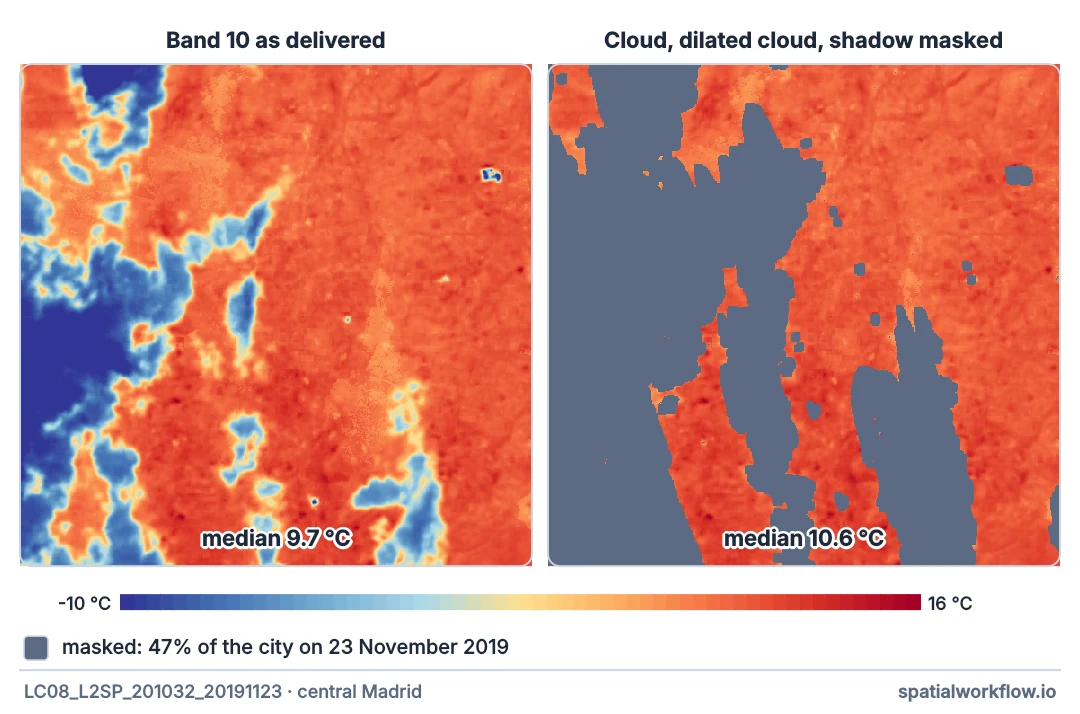
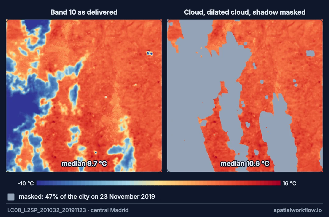
qa_pixel — 47% of the city — the remaining clear ground has a median of 10.6 °C.Decode QA bits, mask cloud, dilation and shadow
1. Decode the QA bits
qa_pixel is a bit field: bit 1 dilated cloud, bit 2 cirrus (Landsat 8/9), bit 3 cloud, bit 4 cloud shadow, bit 5 snow, bit 7 water. Test bits with shifts, not by comparing values.
2. Mask cloud, its dilation and its shadow
The dilated-cloud flag extends the mask around cloud edges where thin cloud cools pixels partially. Shadows cool the ground for real but not because of what is on it.
3. Filter scenes by local cloud cover
Scene-level eo:cloud_cover describes 185 km of scene. Compute the clear fraction within your area and set a threshold.
4. Composite
Median composites of several masked scenes fill gaps and dampen any remaining missed cloud.
5. Look for outliers
Pixels far below the scene's distribution — below the 1st percentile of clear pixels — deserve a second look for missed cloud.
Scene cloud against cloud over the city
Example 1 — scene cloud cover against cloud over the city
rows = []
for i in items[:40]:
    q = read(i, "qa_pixel")
    rows.append((i.properties["eo:cloud_cover"], cloud_mask(q)[q != 1].mean() * 100))
rows = np.array(rows)
print(f"{len(rows)} scenes: correlation of scene and city cloud cover {np.corrcoef(rows.T)[0, 1]:.2f}")
print(f"scenes under 10% overall but over 10% cloudy over the city: "
      f"{((rows[:, 0] < 10) & (rows[:, 1] > 10)).sum()}")
print(f"scenes over 30% overall but under 5% cloudy over the city: "
      f"{((rows[:, 0] > 30) & (rows[:, 1] < 5)).sum()}")
40 scenes: correlation of scene and city cloud cover 0.87
scenes under 10% overall but over 10% cloudy over the city: 2
scenes over 30% overall but under 5% cloudy over the city: 0
Over these 40 scenes, scene-level and city-level cloud cover track each other well (r = 0.87), but not well enough: two scenes rated under 10% cloud overall were more than 10% cloudy over the city. A filter on scene cloud cover lets exactly those scenes into a composite.
Example 2 — what the dilation adds
core = (((qa >> 3) & 1) | ((qa >> 4) & 1)).astype(bool)
ring = cl & ~core
print(f"core cloud and shadow: {core[qa != 1].mean():.1%} of pixels, median {np.nanmedian(lst[core]):.1f} °C")
print(f"dilation ring only:    {ring[qa != 1].mean():.1%} of pixels, median {np.nanmedian(lst[ring]):.1f} °C")
print(f"clear:                                  median {np.nanmedian(lst[~cl]):.1f} °C")
core cloud and shadow: 44.9% of pixels, median 2.7 °C
dilation ring only: 2.2% of pixels, median 8.4 °C
clear: median 10.6 °C
The ring around cloud is cooler than clear ground but warmer than the cloud: partial cloud and shadow edges. Masking only the core would leave these slightly cool pixels in the data.
Example 3 — a composite with and without masking
stack_raw, stack_masked = [], []
same_path = [x for x in items if x.properties["landsat:wrs_path"] == it.properties["landsat:wrs_path"]
             and x.properties["landsat:wrs_row"] == it.properties["landsat:wrs_row"]]   # one pixel grid
for i in [x for x in same_path if x.datetime.year == 2023 and x.datetime.month in (6, 7, 8)]:
    d = read(i, "lwir11").astype("float32")
    q = read(i, "qa_pixel")
    t = np.where(d == 0, np.nan, d * 0.00341802 + 149.0 - 273.15)
    stack_raw.append(t)
    stack_masked.append(np.where(cloud_mask(q), np.nan, t))
h = min(a.shape[0] for a in stack_raw); w = min(a.shape[1] for a in stack_raw)   # guard against a one-pixel rounding difference
raw = np.nanmedian([a[:h, :w] for a in stack_raw], axis=0)
masked = np.nanmedian([a[:h, :w] for a in stack_masked], axis=0)
diff = masked - raw
print(f"{len(stack_raw)} summer scenes; median composite difference {np.nanmedian(diff):+.2f} °C, "
      f"largest {np.nanmax(diff):+.1f} °C")
print(f"pixels where masking changes the composite by more than 2 °C: {(diff > 2).mean():.1%}")
12 summer scenes; median composite difference +1.09 °C, largest +8.1 °C
pixels where masking changes the composite by more than 2 °C: 29.0%
A median composite resists occasional cloud — the median ignores a minority of cold values — but not entirely. Even in a mostly clear summer, masking raises the composite by a median of 1.1 °C and by more than 2 °C on 29% of pixels, up to 8 °C where cloud recurred. Unmasked, those pixels become false cool spots.
Why clouds read cold
Why clouds are cold in LST
The thermal band measures radiation from whatever is at the top of the view. Cloud tops are kilometres up where the air is far colder than the ground. The surface temperature algorithm assumes it is seeing the surface and converts that cold radiance into a cold "surface".
Why thin cloud is harder
Thin cirrus and cloud edges transmit some surface radiation and add their own cold emission. The result is a pixel a few degrees too cool — plausible enough to pass as a shaded street or park.
Why shadows must be masked too
A cloud shadow really is cooler ground: it has been shaded for a while. But it is cool because of the weather that day, not because of what is on the ground, so it misleads any study of land cover and heat.
Missed clouds, bright roofs and snow
- Fmask misses: the QA mask is automated and misses some thin cloud; outlier checks catch part of the rest.
- Bright roofs can be flagged as cloud in some scenes; compare with other dates before removing them from analysis.
- Snow (bit 5) is also cold; winter composites must mask it.
- Water (bit 7) is not cloud; keep or mask it according to the study.
- MODIS has its own QC band with different bit meanings.
Internal links
- How to build a summer LST composite — masking and compositing together
- Cloud masking explained — the general technique
- LST values on the wrong scale — the other source of absurd values
- LST scenes are not comparable — mixing days
- How to read Landsat surface temperature — reading the QA band
- Land surface temperature explained — what the thermal band sees
FAQ
Why are there cold spots in my LST map?
Usually unmasked cloud, cloud edges or cloud shadow.
Which QA bits mark cloud in Landsat Collection 2?
Bit 1 dilated cloud, bit 2 cirrus, bit 3 cloud, bit 4 cloud shadow in qa_pixel.
Is scene cloud cover enough to select scenes?
No. Compute the clear fraction within your area of interest.
Does a median composite remove clouds?
It reduces their influence but does not remove recurring or widespread cloud; mask first.
Should I mask cloud shadow?
Yes; shadows are cool for reasons unrelated to the land surface.
What if clouds are missed by the QA band?
Flag pixels far below the scene's clear-sky distribution and check them against other dates.