LST Resolution Misread

Problem statement

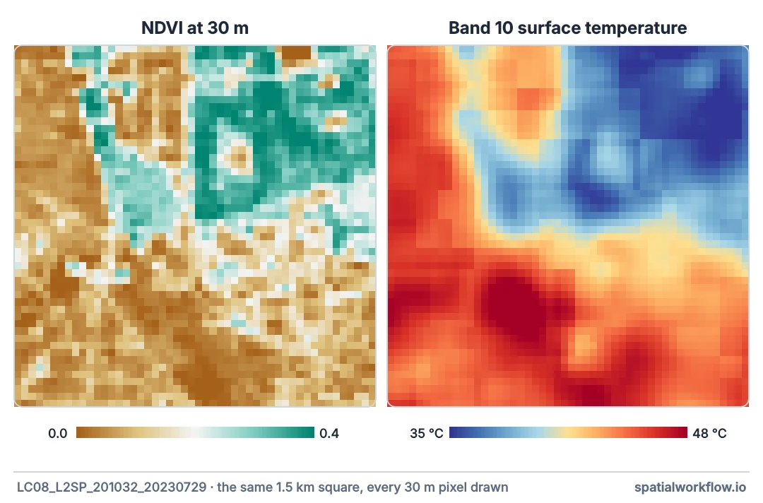
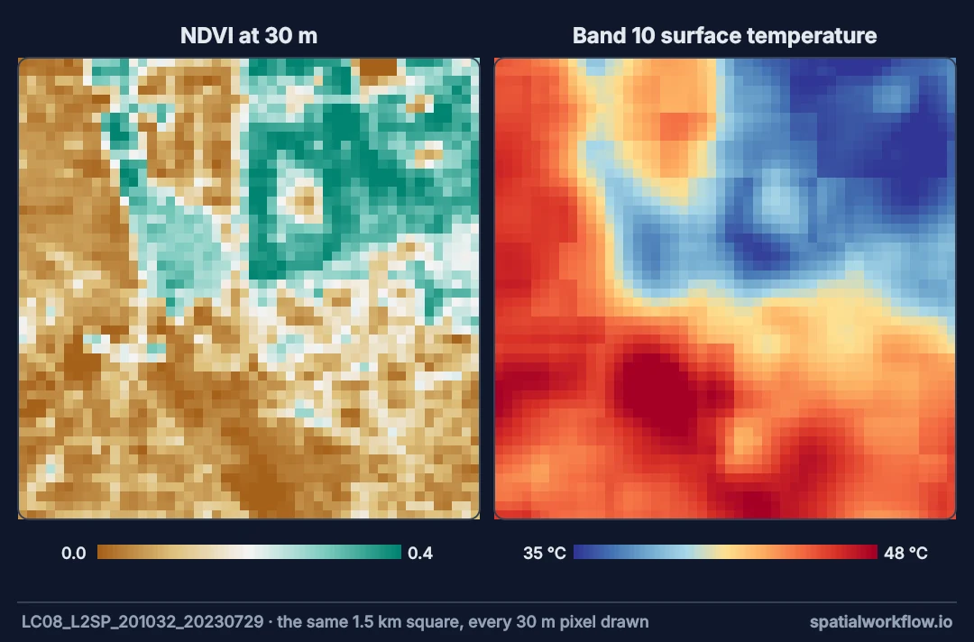
A Landsat surface temperature file has 30 m pixels, so it looks like a 30 m map. It is not. The thermal sensor on Landsat 8 and 9 measures 100 m footprints; the product is resampled to 30 m to line up with the optical bands. Every 30 m pixel carries information blended from roughly a 100 m neighbourhood. Analyses that treat it as 30 m — the temperature of one street tree, one roof, one small square — read the neighbourhood as if it were the feature.

The symptoms are specific: small green spaces look barely cooler than their surroundings, edges are soft over three or four pixels, and correlations with 10 m land cover are weaker than the physics suggests.

Quick answer

Treat Landsat 8/9 LST as 100 m data delivered on a 30 m grid. Aggregate to 90–100 m for analysis, and do not draw conclusions about features smaller than about 200 m across.

import numpy as np, rasterio, pystac_client, planetary_computer
from rasterio.warp import transform_bounds, reproject, Resampling
from scipy import ndimage

AOI = (-3.75, 40.38, -3.63, 40.47)
cat = pystac_client.Client.open("https://planetarycomputer.microsoft.com/api/stac/v1")
it = min((i for i in cat.search(collections=["landsat-c2-l2"], bbox=list(AOI),
                                datetime="2023-07-01/2023-07-31").items()
          if i.properties["platform"] in ("landsat-8", "landsat-9")),
         key=lambda i: i.properties["eo:cloud_cover"])

def read(asset):
    with rasterio.open(planetary_computer.sign(it.assets[asset].href)) as src:
        win = rasterio.windows.from_bounds(*transform_bounds("EPSG:4326", src.crs, *AOI), src.transform).round_offsets().round_lengths()
        return src.read(1, window=win).astype("float64"), src.window_transform(win), src.crs

dn, tf, crs = read("lwir11")
lst = np.where(dn == 0, np.nan, dn * 0.00341802 + 149.0 - 273.15)
red, _, _ = read("red")
nir, _, _ = read("nir08")
ndvi = (nir - red) / (nir + red)                                   # a band measured at 30 m

def lag_corr(a, k):
    ok = np.isfinite(a[:, :-k]) & np.isfinite(a[:, k:])
    return np.corrcoef(a[:, :-k][ok], a[:, k:][ok])[0, 1]

print(f"{it.id}")
for k in (1, 2, 3, 4, 6):
    print(f"pixels {k * 30:>3} m apart: correlation LST {lag_corr(lst, k):.2f}, NDVI {lag_corr(ndvi, k):.2f}")

LC08_L2SP_201032_20230729_02_T1
pixels  30 m apart: correlation LST 0.98, NDVI 0.79
pixels  60 m apart: correlation LST 0.94, NDVI 0.60
pixels  90 m apart: correlation LST 0.88, NDVI 0.50
pixels 120 m apart: correlation LST 0.81, NDVI 0.44
pixels 180 m apart: correlation LST 0.68, NDVI 0.37

Neighbouring LST pixels are far more alike than neighbouring NDVI pixels, and they stay alike for three or four pixels. That is the signature of a coarser measurement resampled onto a finer grid.

Native resolution, aggregation, matched land cover

1. Know the native resolution

Landsat 8/9 TIRS: 100 m. Landsat 7 ETM+: 60 m. Landsat 5 TM: 120 m. MODIS: 1 km. ECOSTRESS: about 70 m.

2. Aggregate before analysis

Average LST to 90 m (3 × 3 Landsat pixels) or 100 m. Statistics on 30 m pixels count the same information nine times over.

3. Match land cover to the same scale

Use the share of each class within each 90–100 m cell, not the class of a 10 m or 30 m pixel.

4. Keep small features out of conclusions

A 50 m pocket park is a fraction of one thermal footprint. Its "temperature" is mostly its surroundings.

5. Account for spatial autocorrelation

Tests that assume independent pixels overstate significance by a large factor at 30 m.

Small tree patches and soft edges

Example 1 — small tree patches look warm

wc = np.zeros(lst.shape, dtype="uint8")
wc_item = next(cat.search(collections=["esa-worldcover"], bbox=list(AOI), datetime="2021").items())
with rasterio.open(planetary_computer.sign(wc_item.assets["map"].href)) as src:
    reproject(rasterio.band(src, 1), wc, dst_transform=tf, dst_crs=crs, resampling=Resampling.mode)
trees = wc == 10
lab, n = ndimage.label(trees)
size = np.bincount(lab.ravel())[lab] * 0.09                          # hectares of the patch each pixel belongs to
built = np.nanmedian(lst[wc == 50])
for lo, hi in ((0, 0.5), (0.5, 2), (2, 10), (10, 1e9)):
    m = trees & (size >= lo) & (size < hi) & np.isfinite(lst)
    print(f"tree patches {lo:>4}–{hi if hi < 1e9 else '∞':<4} ha: {m.sum():>6,} px, "
          f"median {np.median(lst[m]):5.1f} °C ({np.median(lst[m]) - built:+.1f} vs built-up)")

tree patches    0–0.5  ha:  3,619 px, median  43.3 °C (-1.0 vs built-up)
tree patches  0.5–2    ha:  3,332 px, median  42.7 °C (-1.6 vs built-up)
tree patches    2–10   ha:  4,879 px, median  42.4 °C (-1.9 vs built-up)
tree patches   10–∞    ha: 11,568 px, median  41.6 °C (-2.7 vs built-up)

Small tree patches look only slightly cooler than built-up land; large ones look much cooler. Part of that is real — large parks are cooler — but for patches under a hectare most of the difference is that their pixels are measuring the streets around them.

Example 2 — how soft an edge is

big = trees & (size >= 10)
d_in = ndimage.distance_transform_edt(big) * 30
d_out = ndimage.distance_transform_edt(~big) * 30
dist = np.where(big, -d_in, d_out)                                    # negative inside the patch
for lo in range(-150, 180, 30):
    m = (dist >= lo) & (dist < lo + 30) & np.isfinite(lst)
    print(f"{lo:>5} to {lo + 30:>4} m from the edge: LST {np.median(lst[m]):5.1f} °C, NDVI {np.nanmedian(ndvi[m]):.2f}")

 -150 to -120 m from the edge: LST  36.5 °C, NDVI 0.32
 -120 to  -90 m from the edge: LST  37.9 °C, NDVI 0.32
  -90 to  -60 m from the edge: LST  40.3 °C, NDVI 0.28
  -60 to  -30 m from the edge: LST  41.6 °C, NDVI 0.25
  -30 to    0 m from the edge: LST  42.3 °C, NDVI 0.21
    0 to   30 m from the edge: LST   nan °C, NDVI nan
   30 to   60 m from the edge: LST  43.0 °C, NDVI 0.15
   60 to   90 m from the edge: LST  43.7 °C, NDVI 0.13
   90 to  120 m from the edge: LST  43.9 °C, NDVI 0.13
  120 to  150 m from the edge: LST  44.0 °C, NDVI 0.12
  150 to  180 m from the edge: LST  44.1 °C, NDVI 0.13

Neither edge is sharp. NDVI falls steadily across the boundary as the canopy thins towards it. Surface temperature rises by 5.8 °C over the last 150 m inside the patch and levels off within about 90 m outside. The part inside is largely real: the interior of a large tree patch is cooler than its sunlit, street-facing edge. The 100 m thermal footprint smears the last pixel or two on each side, and that smear is what a 30 m analysis would misread as cooling reaching into the streets. (The empty 0–30 m band is an artefact of the distance transform: the first pixel outside sits 30 m from the nearest tree pixel.)

Example 3 — aggregating loses little

h, w = (lst.shape[0] // 3) * 3, (lst.shape[1] // 3) * 3
agg = np.nanmean(lst[:h, :w].reshape(h // 3, 3, w // 3, 3), axis=(1, 3))
back = np.repeat(np.repeat(agg, 3, axis=0), 3, axis=1)
ndvi_agg = np.nanmean(ndvi[:h, :w].reshape(h // 3, 3, w // 3, 3), axis=(1, 3))
ndvi_back = np.repeat(np.repeat(ndvi_agg, 3, axis=0), 3, axis=1)
kept = lambda full, coarse: 1 - np.nanvar(full[:h, :w] - coarse) / np.nanvar(full[:h, :w])
print(f"variance kept at 90 m: LST {kept(lst, back):.0%}, NDVI {kept(ndvi, ndvi_back):.0%}")

variance kept at 90 m: LST 96%, NDVI 71%

Averaging LST to 90 m keeps nearly all its variance; averaging NDVI does not. There was little 30 m detail in the LST to lose.

Why delivered pixels are not sensor footprints

Why the product is delivered at 30 m

Resampling thermal data to the optical grid makes it easy to combine with reflectance bands and land cover, and to process a whole scene with one grid. It does not create detail: cubic convolution interpolates between 100 m measurements.

Why the sensor footprint is larger than the pixel spacing

A detector's footprint also has soft edges: its point spread function gives weight to radiation from beyond its nominal pixel. The effective footprint is broader than 100 m, which is why autocorrelation persists beyond three pixels.

Why small green spaces are underestimated

A pixel centred on a 40 m park integrates the park and a large ring of surrounding streets. Its temperature is a weighted mix leaning towards the streets. Physical measurements on the ground usually show a larger cooling within small parks than Landsat does.

Sharpening, ECOSTRESS and MODIS

• Sharpening methods (thermal downscaling with NDVI or impervious fraction) produce 30 m estimates, but they are models, not measurements.
• ECOSTRESS at about 70 m and airborne thermal surveys at 1–5 m resolve smaller features.
• MODIS 1 km is far coarser still; whole districts share one pixel.
• Validation of LST with point measurements must account for footprint mismatch.
• Statistics: effective sample size at 30 m is roughly one-ninth to one-eleventh of the pixel count.

Internal links

• Landsat thermal data explained — native resolutions by sensor
• How to measure the cooling effect of parks — where edges matter most
• Urban cooling and green space explained — small and large green spaces
• How to relate LST to vegetation — matching scales
• Raster resampling explained — aggregation methods
• Land surface temperature explained — what a pixel measures

FAQ

What is the real resolution of Landsat LST?

100 m for Landsat 8 and 9, delivered at 30 m.

Can I measure the temperature of a single street tree?

Not with Landsat; the tree is a small fraction of one thermal footprint.

Should I aggregate LST before analysis?

Yes, to 90–100 m, with land cover summarised to the same cells.

Why are my small parks not cooler?

Their pixels also measure the surrounding streets; the cooling is diluted.

Does thermal sharpening solve this?

It produces modelled 30 m estimates, not measurements; treat them with care.

What data resolves small features?

Airborne thermal surveys, and to a lesser degree ECOSTRESS at about 70 m.