Urban Cooling and Green Space Explained

On this page

Problem statement

Planting trees is the most common prescription for urban heat, and the evidence that green space cools is overwhelming. What the evidence says in detail matters for how the prescription is filled. Trees cool mostly through shade and transpiration; grass cools only while it is watered; the cooling of a park extends beyond its edge by a distance that depends on its size; and in a dry summer an unirrigated lawn can be almost as hot as a car park. "More green" measured as NDVI or green area is a proxy that blends all of these.

Understanding the mechanisms tells you which kind of green, where and how much — and how to read the satellite evidence without overstating it.

Quick answer

Green space cools by:

Shade — trees intercept sunlight before it reaches the ground.
Evapotranspiration — water evaporated from leaves and soil uses energy that would otherwise heat the surface.
Altered surfaces — soil and vegetation store less heat than masonry and release it faster at night.

import numpy as np, rasterio, pystac_client, planetary_computer
from rasterio.warp import reproject, Resampling

with rasterio.open("madrid_lst_jja2023.tif") as src:              # from the composite guide
    lst = src.read(1)
    tf, crs, shape = src.transform, src.crs, (src.height, src.width)
cat = pystac_client.Client.open("https://planetarycomputer.microsoft.com/api/stac/v1")
wc = np.zeros(shape, dtype="uint8")
for it in cat.search(collections=["esa-worldcover"], bbox=[-4.05, 40.20, -3.35, 40.65], datetime="2021").items():
    with rasterio.open(planetary_computer.sign(it.assets["map"].href)) as src:
        tmp = np.zeros(shape, dtype="uint8")
        reproject(rasterio.band(src, 1), tmp, dst_transform=tf, dst_crs=crs, resampling=Resampling.mode)
        wc = np.where(wc == 0, tmp, wc)

# 300 m blocks (10 × 10 pixels) inside the city: tree share against median LST
k = 10
h, w = (shape[0] // k) * k, (shape[1] // k) * k
blk = lambda a: a[:h, :w].reshape(h // k, k, w // k, k)
tree = (blk(wc == 10)).mean(axis=(1, 3))
built = (blk(wc == 50)).mean(axis=(1, 3))
water = (blk(wc == 80)).mean(axis=(1, 3))
t = np.nanmedian(blk(lst), axis=(1, 3))
city = (built + tree >= 0.8) & (water < 0.05) & np.isfinite(t)       # blocks of buildings and trees
slope, icpt = np.polyfit(tree[city], t[city], 1)
print(f"{city.sum():,} urban blocks of 300 m")
print(f"median LST falls by {-slope / 10:.2f} °C for every 10 points of tree cover "
      f"(from {icpt:.1f} °C at no trees)")
for lo, hi in ((0, 0.1), (0.1, 0.3), (0.3, 0.6), (0.6, 1.01)):
    m = city & (tree >= lo) & (tree < hi)
    print(f"tree share {lo:.0%}–{min(hi, 1):.0%}: {m.sum():>5} blocks, median LST {np.median(t[m]):5.1f} °C")

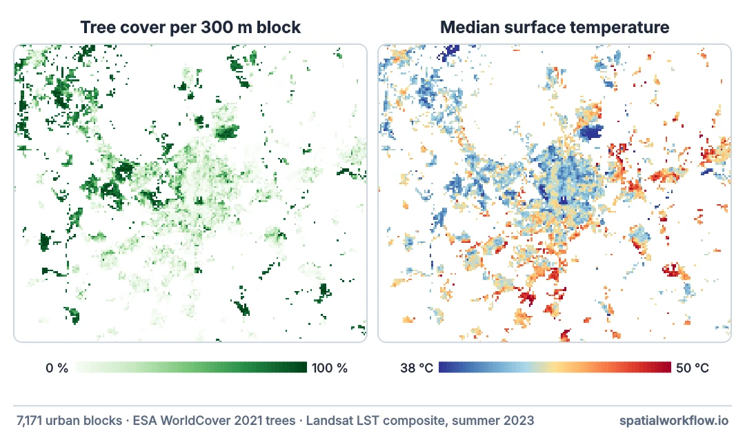
7,171 urban blocks of 300 m
median LST falls by 0.41 °C for every 10 points of tree cover (from 44.7 °C at no trees)
tree share 0%–10%:  2698 blocks, median LST  44.7 °C
tree share 10%–30%:  1628 blocks, median LST  43.2 °C
tree share 30%–60%:   951 blocks, median LST  42.0 °C
tree share 60%–100%:  1894 blocks, median LST  41.5 °C

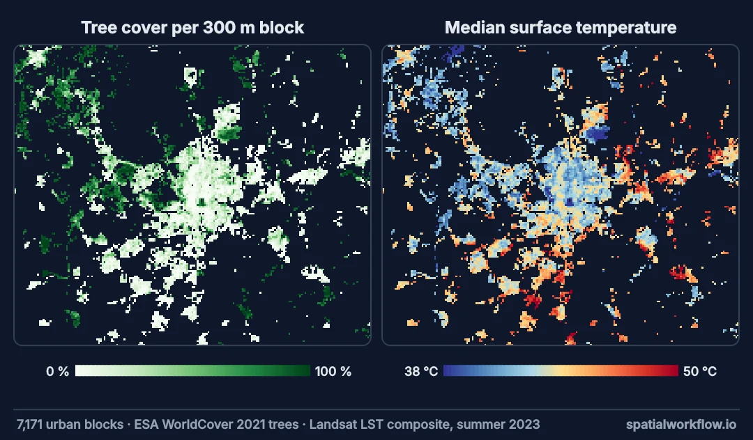
Among 7,171 urban blocks — mixes of buildings and trees — the median surface temperature falls steadily from 44.7 °C with almost no trees to 41.5 °C where trees cover most of the block, about 0.4 °C for every ten points of canopy. The effect is large enough to matter for a street, and it is a relationship between blocks, not a measured effect of planting.

Two block maps of Madrid side by side: tree cover per 300 metre block in greens on the left, median summer surface temperature per block on the right. Blocks with many trees are among the coolest on the right. — The 7,171 urban blocks, tree share on the left and summer surface temperature on the right. The wooded blocks — the big parks and the woodland on the western edge — are the blue ones on the right; the hottest blocks lie at the eastern and southern edges, where there are almost no trees. Side by side, the 0.4 °C per ten points of canopy is visible block by block.

Trees, grass, water, size and surface versus air

1. Separate trees from grass

Trees provide shade and deep-rooted transpiration; grass provides only surface evaporation, and only while the soil is moist. Measures that lump them (green area, NDVI) blur the difference.

2. Consider water

Irrigation keeps grass cool in a dry summer. Without it, grass browns and heats. The cooling of urban lawns is partly a water bill.

3. Consider size and shape

Large parks form cool islands with measurable reach into surrounding streets. Small parks and street trees cool mostly their own footprint and shade. Many small patches spread through a district can matter as much as one large park.

4. Distinguish surface and air cooling

Satellite LST shows large surface differences. Air temperature differences are smaller — typically one to a few degrees — and most pronounced at night and in still weather.

5. Read correlation as correlation

Greener neighbourhoods differ from others in building age, density, income and more. Cross-sectional LST–green relationships are evidence of association; before-and-after studies of planting estimate effects.

Shade, water and surface: the three ways green space cools.

Trees against grass in a dry Madrid summer

The data used on this page

The summer 2023 land surface temperature composite of Madrid from the composite guide: the median of every Landsat 8 and 9 Collection 2 Level-2 scene from June to August 2023 on the Microsoft Planetary Computer with more than a fifth of the area clear, on a 30 m UTM 30N grid, with the count of clear observations as a second band. The setup rebuilds it if madrid_lst_jja2023.tif is missing.

import os

import numpy as np
import planetary_computer
import pystac_client
import rasterio
from rasterio.transform import from_origin
from rasterio.warp import Resampling, reproject, transform_bounds

if not os.path.exists("madrid_lst_jja2023.tif"):        # the composite guide's code, without the prints
    AOI = (-4.05, 40.20, -3.35, 40.65)
    DST_CRS = "EPSG:32630"
    x0, y0, x1, y1 = transform_bounds("EPSG:4326", DST_CRS, *AOI)
    x0, y1 = np.floor(x0 / 30) * 30, np.ceil(y1 / 30) * 30
    W, H = int(np.ceil((x1 - x0) / 30)), int(np.ceil((y1 - y0) / 30))
    DST_TF = from_origin(x0, y1, 30, 30)
    cat = pystac_client.Client.open("https://planetarycomputer.microsoft.com/api/stac/v1")
    items = [i for i in cat.search(collections=["landsat-c2-l2"], bbox=list(AOI),
                                   datetime="2023-06-01/2023-08-31").items()
             if i.properties["platform"] in ("landsat-8", "landsat-9") and i.properties["eo:cloud_cover"] < 60]

    def on_grid(item, asset):
        out = np.zeros((H, W), dtype="uint16")
        with rasterio.open(planetary_computer.sign(item.assets[asset].href)) as src:
            reproject(rasterio.band(src, 1), out, dst_transform=DST_TF, dst_crs=DST_CRS,
                      resampling=Resampling.nearest, src_nodata=0 if asset == "lwir11" else 1, dst_nodata=0)
        return out

    layers = []
    for it in sorted(items, key=lambda i: i.datetime):
        dn, qa = on_grid(it, "lwir11"), on_grid(it, "qa_pixel")
        t = np.where(dn == 0, np.nan, dn * 0.00341802 + 149.0 - 273.15)
        t[(((qa >> 1) & 1) | ((qa >> 3) & 1) | ((qa >> 4) & 1)) == 1] = np.nan
        if np.isfinite(t).mean() > 0.2:
            layers.append(t)
    stack = np.stack(layers)
    profile = {"driver": "GTiff", "height": H, "width": W, "count": 2, "dtype": "float32",
               "crs": DST_CRS, "transform": DST_TF, "nodata": np.nan, "compress": "deflate"}
    with rasterio.open("madrid_lst_jja2023.tif", "w", **profile) as dst:
        dst.write(np.nanmedian(stack, axis=0).astype("float32"), 1)
        dst.write(np.isfinite(stack).sum(axis=0).astype("float32"), 2)
        dst.set_band_description(1, "median LST °C, Landsat 8/9, Jun–Aug 2023")
        dst.set_band_description(2, "clear observations")
with rasterio.open("madrid_lst_jja2023.tif") as src:
    print(src.shape, src.crs, src.descriptions or "", f"median {np.nanmedian(src.read(1)):.1f} °C")

(1682, 1994) EPSG:32630 ('median LST °C, Landsat 8/9, Jun–Aug 2023', 'clear observations') median 46.9 °C

Example 1 — trees against grass in a dry summer

ok = np.isfinite(lst)
for code, name in ((10, "tree cover"), (30, "grassland"), (50, "built-up"), (60, "bare")):
    m = ok & (wc == code)
    print(f"{name:<11} median LST {np.nanmedian(lst[m]):5.1f} °C")

tree cover  median LST  43.1 °C
grassland   median LST  48.0 °C
built-up    median LST  44.7 °C
bare        median LST  46.2 °C

Grassland around Madrid in July and August is largely unirrigated and dry: its surface is hot, often hotter than the city. Tree cover is the cool class. "Green" is not one thing in a Mediterranean summer.

Example 2 — does the relationship hold within densities?

for lo, hi in ((0.3, 0.6), (0.6, 0.8)):
    m = city & (built >= lo) & (built < hi)
    s_, _ = np.polyfit(tree[m], t[m], 1)
    print(f"blocks {lo:.0%}–{hi:.0%} built-up: {m.sum():>4} blocks, "
          f"{-s_ / 10:.2f} °C cooler per 10 points of tree cover")

blocks 30%–60% built-up:  853 blocks, 0.68 °C cooler per 10 points of tree cover
blocks 60%–80% built-up: 1251 blocks, 1.30 °C cooler per 10 points of tree cover

Holding the built-up share roughly constant, more trees still go with cooler blocks — and more strongly than the citywide slope suggests: 0.7 °C per ten points of canopy in moderately built-up blocks, 1.3 °C in the densest. Trees matter most where there is least of anything else to cool the surface. That is closer to the question a planner asks — what trees add to a given kind of street — than the citywide slope.

Example 3 — the coolest built-up blocks

bb = city & (built >= 0.6)
cool = bb & (t <= np.percentile(t[bb], 10))
hot = bb & (t >= np.percentile(t[bb], 90))
print(f"dense blocks, coolest 10%: tree share {tree[cool].mean():.0%}; "
      f"hottest 10%: tree share {tree[hot].mean():.0%}")

dense blocks, coolest 10%: tree share 21%; hottest 10%: tree share 2%

Among the most built-up blocks, the coolest tenth has ten times the tree cover of the hottest tenth — 21% against 2%. Other factors — street width, roof colour, water — make up the rest of the difference.

Urban blocks by tree cover: more canopy, cooler surfaces.

Why trees beat grass, and evidence is correlational

Why trees beat grass

A tree's canopy shades the ground and its roots reach water that surface grasses cannot, so it keeps transpiring in dry spells. Its leaves are cooled by transpiration and by air flowing through the canopy. A lawn in drought has neither shade nor water to evaporate; its surface heats like bare soil.

Why cooling extends beyond parks

Cool, dense air over a large park drains into surrounding streets on calm nights; shade from edge trees reaches pavements. The reach grows with park size and falls off within a few hundred metres. For surface temperature at Landsat resolution, part of the apparent reach is the 100 m pixel straddling the edge.

Why the evidence is mostly correlational

Neighbourhoods were not assigned tree cover at random. Older, wealthier or less dense districts often have more trees and other differences in materials and layout. Controlling for built-up density helps; longitudinal studies of new plantings, and physical models, are needed for causal estimates.

Holding density constant, the tree effect is larger, not smaller.

Water use, nights and humidity

Water use: irrigated greenery in dry cities trades water for cooling; drought restrictions reverse the cooling.
Night-time: dense tree canopy can trap heat under it at night in some street geometries.
Humidity: transpiration adds humidity, which lowers the benefit for thermal comfort in humid climates.
Species and size: large, broad-crowned trees cool far more than young or narrow ones.
Resolution: street trees are small relative to 100 m thermal pixels; their effect is diluted in satellite LST.

Internal links

How to measure the cooling effect of parks — distance profiles
How to relate LST to vegetation — pixel-level relationships
Surface urban heat island explained — the city-scale pattern
How to calculate NDVI in Python — the common green proxy
Heat exposure explained — who benefits from cooling
Urban morphology explained — the built form trees sit among

FAQ

How much do trees cool a city?

Surface temperatures under and near dense tree canopy can be many degrees below paved surfaces; air temperature effects are typically one to a few degrees.

Are grass and trees equally cooling?

No. Trees shade and keep transpiring in drought; grass cools only while watered.

How far does a park's cooling reach?

Typically up to a few hundred metres for large parks, less for small ones.

Is NDVI a good measure of cooling vegetation?

A rough one; it does not distinguish trees from grass or watered from dry vegetation.

Does satellite data prove that planting trees cools streets?

It shows strong associations; controlled comparisons and before-and-after studies are needed for causal estimates.

Why is dry grass hot?

Without water to evaporate, absorbed sunlight goes into heating the surface, as with bare soil.