SUHI Rural Reference Gives the Wrong Answer

Problem statement

Your surface urban heat island comes out at +6 °C, a colleague's for the same city and summer at −2 °C, and neither calculation has a bug. The urban side of the subtraction is fairly stable; the rural side is whatever the analyst decided "surroundings" means. A ring that is mostly dry cropland, one that is mostly forest, one that reaches up into mountains or includes a reservoir — each gives a different reference temperature, and the heat island inherits the whole difference.

The rural reference is the least discussed choice in a SUHI calculation and usually the one that moves the answer most.

Quick answer

Compute the SUHI with several defensible rural references and report the range. Exclude water and land far above or below the city's elevation; state the land cover of the reference.

import numpy as np, rasterio, pystac_client, planetary_computer
from rasterio.warp import reproject, Resampling
from scipy import ndimage

with rasterio.open("madrid_lst_jja2023.tif") as src:              # from the composite guide
    lst, count = src.read(1), src.read(2)
    tf, crs, shape = src.transform, src.crs, (src.height, src.width)
cat = pystac_client.Client.open("https://planetarycomputer.microsoft.com/api/stac/v1")

def on_grid(collection, asset, resampling, dtype, **search):
    out = np.zeros(shape, dtype=dtype)
    for it in cat.search(collections=[collection], bbox=[-4.05, 40.20, -3.35, 40.65], **search).items():
        tmp = np.zeros(shape, dtype=dtype)
        with rasterio.open(planetary_computer.sign(it.assets[asset].href)) as src:
            reproject(rasterio.band(src, 1), tmp, dst_transform=tf, dst_crs=crs, resampling=resampling)
        out = np.where(out == 0, tmp, out)
    return out

wc = on_grid("esa-worldcover", "map", Resampling.mode, "uint8", datetime="2021")
dem = on_grid("cop-dem-glo-30", "data", Resampling.bilinear, "float32")

urban = wc == 50
lab, _ = ndimage.label(urban)
city = ndimage.binary_closing(lab == np.bincount(lab.ravel())[1:].argmax() + 1, iterations=10)
dist = ndimage.distance_transform_edt(~city) * 30 / 1000
valid = np.isfinite(lst) & (count >= 3)
u = np.nanmedian(lst[city & urban & valid])
city_elev = np.median(dem[city & urban])
print(f"urban median LST {u:.1f} °C at a median elevation of {city_elev:.0f} m")

ring = (dist > 5) & (dist <= 15) & valid & ~urban
refs = {
    "ring 5–15 km, anything unbuilt": ring,
    "ring 5–15 km, no water": ring & (wc != 80),
    "ring, no water, within ±100 m of city": ring & (wc != 80) & (abs(dem - city_elev) <= 100),
    "ring, cropland only": ring & (wc == 40),
    "ring, grassland only": ring & (wc == 30),
    "ring, tree cover only": ring & (wc == 10),
}
for name, m in refs.items():
    r = np.nanmedian(lst[m])
    print(f"{name:<40} {m.sum():>8,} px  rural {r:5.1f} °C  SUHI {u - r:+5.1f} °C")

urban median LST 44.4 °C at a median elevation of 648 m
ring 5–15 km, anything unbuilt            637,594 px  rural  47.9 °C  SUHI  -3.5 °C
ring 5–15 km, no water                    629,436 px  rural  48.0 °C  SUHI  -3.6 °C
ring, no water, within ±100 m of city     443,888 px  rural  48.3 °C  SUHI  -3.9 °C
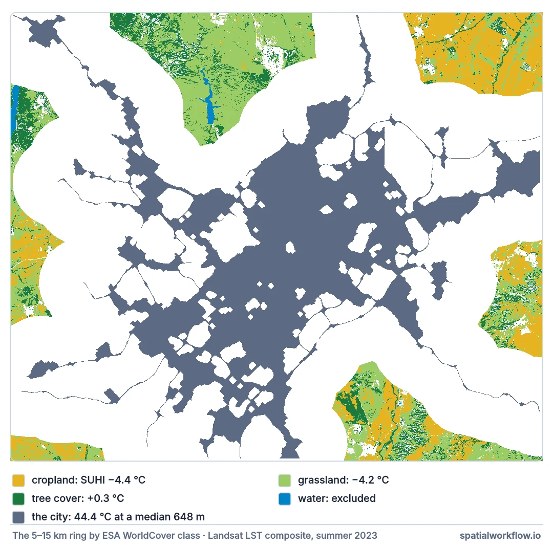
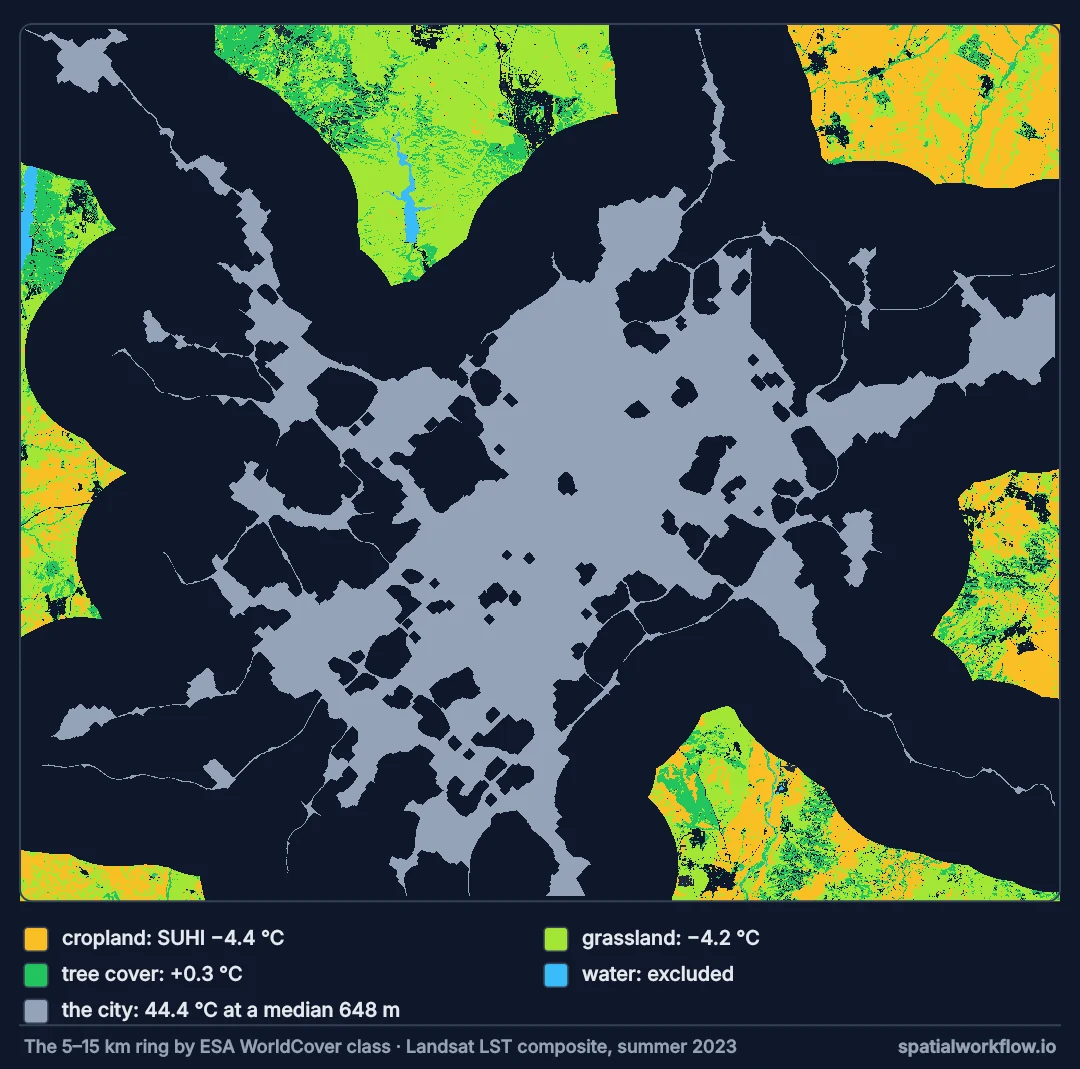
ring, cropland only                       209,657 px  rural  48.8 °C  SUHI  -4.4 °C
ring, grassland only                      298,063 px  rural  48.6 °C  SUHI  -4.2 °C
ring, tree cover only                     102,677 px  rural  44.1 °C  SUHI  +0.3 °C

The same urban temperature, six rural references, a spread of 4.7 °C in the heat island, from −4.4 °C against cropland to +0.3 °C against woodland — a change of sign that depends only on what the analyst called rural.

Remove water, limit elevation, test several rings

1. Remove water

Reservoirs and rivers are cool in summer daytime and warm at night. Any water in the reference biases it.

2. Limit elevation difference

Surface temperature falls with altitude. Keep the reference within about 100 m of the city's elevation, or correct for a lapse rate.

3. Report the land cover of the reference

Dry cropland, grassland and forest have very different summer surface temperatures. Say which the reference is — or match it to what the city replaced.

4. Test several rings

Near rings may still be influenced by the city; far rings reach different climates or terrain. The spread across rings is part of the uncertainty.

5. Report a range

A single SUHI number hides the reference choice. Give the range across defensible references along with the preferred value.

The reference by ring and by direction

The data used on this page

The summer 2023 land surface temperature composite of Madrid from the composite guide: the median of every Landsat 8 and 9 Collection 2 Level-2 scene from June to August 2023 on the Microsoft Planetary Computer with more than a fifth of the area clear, on a 30 m UTM 30N grid, with the count of clear observations as a second band. The setup rebuilds it if madrid_lst_jja2023.tif is missing.

import os

import numpy as np
import planetary_computer
import pystac_client
import rasterio
from rasterio.transform import from_origin
from rasterio.warp import Resampling, reproject, transform_bounds

if not os.path.exists("madrid_lst_jja2023.tif"):        # the composite guide's code, without the prints
    AOI = (-4.05, 40.20, -3.35, 40.65)
    DST_CRS = "EPSG:32630"
    x0, y0, x1, y1 = transform_bounds("EPSG:4326", DST_CRS, *AOI)
    x0, y1 = np.floor(x0 / 30) * 30, np.ceil(y1 / 30) * 30
    W, H = int(np.ceil((x1 - x0) / 30)), int(np.ceil((y1 - y0) / 30))
    DST_TF = from_origin(x0, y1, 30, 30)
    cat = pystac_client.Client.open("https://planetarycomputer.microsoft.com/api/stac/v1")
    items = [i for i in cat.search(collections=["landsat-c2-l2"], bbox=list(AOI),
                                   datetime="2023-06-01/2023-08-31").items()
             if i.properties["platform"] in ("landsat-8", "landsat-9") and i.properties["eo:cloud_cover"] < 60]

    def on_grid(item, asset):
        out = np.zeros((H, W), dtype="uint16")
        with rasterio.open(planetary_computer.sign(item.assets[asset].href)) as src:
            reproject(rasterio.band(src, 1), out, dst_transform=DST_TF, dst_crs=DST_CRS,
                      resampling=Resampling.nearest, src_nodata=0 if asset == "lwir11" else 1, dst_nodata=0)
        return out

    layers = []
    for it in sorted(items, key=lambda i: i.datetime):
        dn, qa = on_grid(it, "lwir11"), on_grid(it, "qa_pixel")
        t = np.where(dn == 0, np.nan, dn * 0.00341802 + 149.0 - 273.15)
        t[(((qa >> 1) & 1) | ((qa >> 3) & 1) | ((qa >> 4) & 1)) == 1] = np.nan
        if np.isfinite(t).mean() > 0.2:
            layers.append(t)
    stack = np.stack(layers)
    profile = {"driver": "GTiff", "height": H, "width": W, "count": 2, "dtype": "float32",
               "crs": DST_CRS, "transform": DST_TF, "nodata": np.nan, "compress": "deflate"}
    with rasterio.open("madrid_lst_jja2023.tif", "w", **profile) as dst:
        dst.write(np.nanmedian(stack, axis=0).astype("float32"), 1)
        dst.write(np.isfinite(stack).sum(axis=0).astype("float32"), 2)
        dst.set_band_description(1, "median LST °C, Landsat 8/9, Jun–Aug 2023")
        dst.set_band_description(2, "clear observations")
with rasterio.open("madrid_lst_jja2023.tif") as src:
    print(src.shape, src.crs, src.descriptions or "", f"median {np.nanmedian(src.read(1)):.1f} °C")

(1682, 1994) EPSG:32630 ('median LST °C, Landsat 8/9, Jun–Aug 2023', 'clear observations') median 46.9 °C

Example 1 — what the ring is made of

names = {10: "tree cover", 20: "shrubland", 30: "grassland", 40: "cropland", 60: "bare", 80: "water"}
m = ring
for code, n in names.items():
    share = (wc[m] == code).mean()
    if share > 0.01:
        print(f"{n:<11} {share:5.1%} of the ring, median LST {np.nanmedian(lst[m & (wc == code)]):5.1f} °C")

tree cover  16.1% of the ring, median LST  44.1 °C
shrubland    2.4% of the ring, median LST  44.6 °C
grassland   46.7% of the ring, median LST  48.6 °C
cropland    32.9% of the ring, median LST  48.8 °C
water        1.3% of the ring, median LST  33.1 °C

An "unbuilt" ring is a mixture: here 47% grassland and 33% cropland, both near 48.7 °C, and 16% tree cover at 44.1 °C. Its median temperature depends on the mixture — which in turn depends on where the city happens to sit.

Example 2 — the reference by direction

rows_, cols_ = np.indices(shape)
cy, cx = [np.median(a[city]) for a in (rows_, cols_)]
angle = np.degrees(np.arctan2(-(rows_ - cy), cols_ - cx)) % 360
for lo, name in ((45, "north"), (135, "west"), (225, "south"), (315, "east")):
    sector = ((angle - lo) % 360 < 90) & refs["ring 5–15 km, no water"]
    print(f"{name:<5}: {np.nanmedian(lst[sector]):5.1f} °C, elevation {np.median(dem[sector]):4.0f} m, "
          f"tree share {(wc[sector] == 10).mean():.0%}")

north:  48.2 °C, elevation  718 m, tree share 18%
west :  47.5 °C, elevation  633 m, tree share 20%
south:  47.2 °C, elevation  585 m, tree share 18%
east :  48.5 °C, elevation  704 m, tree share 10%

The countryside around a city is not uniform: the four sectors differ by 1.3 °C, by 130 m of elevation and by a factor of two in tree share. A reference drawn only from one side — as happens when a study area is clipped — takes that side's land cover and terrain with it.

Example 3 — the city against what it replaced

pre = ring & np.isin(wc, [30, 40])                                     # the open land Madrid expanded into
print(f"SUHI against open farmland and grassland: {u - np.nanmedian(lst[pre]):+.1f} °C")
print(f"SUHI against woodland:                    {u - np.nanmedian(lst[ring & (wc == 10)]):+.1f} °C")

SUHI against open farmland and grassland: -4.3 °C
SUHI against woodland:                    +0.3 °C

The question "how much warmer did building the city make this land?" wants a reference like the land that was built on. Around Madrid that is largely open farmland and grassland, not woodland — and against it the late-morning heat island is −4.3 °C, a cool island.

The reference matters more than the city

Why the reference matters more than the city

The urban temperature is an average over many similar built surfaces. The rural reference averages very different surfaces — irrigated fields, dry pasture, forest, bare soil — whose summer temperatures differ by more than the heat island itself. Small changes in the mix move the reference a lot.

Why daytime SUHI can be negative

In a dry summer, unirrigated grassland and harvested cropland have no water to evaporate and bake in the sun. The city has irrigated parks, trees and building shade. Against such a reference the city is cooler at midday; against woodland it is warmer.

Why elevation must be controlled

Air and surface temperatures fall with altitude — for air about 6.5 °C per kilometre on average. A reference that climbs into nearby hills is cooler for reasons unrelated to urbanisation.

Night-time islands and neighbouring towns

• Night-time SUHI is less sensitive to the reference because rural surfaces converge at night; daytime values are most affected.
• Seasons: harvest turns green cropland to bare stubble in weeks, changing the reference within one summer.
• Neighbouring towns in the ring raise the reference; exclude all built-up land, not just the main city.
• Multi-city studies need one rule applied everywhere, and even then comparisons across climates are loose.
• Air-temperature UHI uses rural stations, which carry their own siting problems.

Internal links

• How to calculate SUHI intensity — the main calculation
• Surface urban heat island explained — day, night and type
• How to build a summer LST composite — the input used here
• Urban extent explained — defining the urban side
• LST scenes are not comparable — other ways SUHI numbers diverge
• Density depends on the boundary — the same problem for density

FAQ

Why is my SUHI negative?

The rural reference is hotter than the city — common in daytime in dry climates where the countryside is dry grass or bare soil.

What should the rural reference be?

Unbuilt land near the city, excluding water, within about 100 m of the city's elevation, with its land cover reported.

How far out should the rural ring be?

Typically a few to a few tens of kilometres beyond the urban edge; test several and report the spread.

Should I include forests in the rural reference?

Only if they represent the surroundings; report the land cover mix so readers can judge.

Does the reference problem affect night-time SUHI?

Less than daytime, but water and elevation still matter.

How do I make SUHI comparable across cities?

Apply one fixed rule everywhere and report the reference land cover; comparisons across climates remain approximate.