How to Read Landsat Surface Temperature in Python

Problem statement

Landsat's Collection 2 Level-2 surface temperature product gives the temperature of the ground — roofs, roads, fields, water — at 30 m for every clear Landsat scene since the 1980s. It is the standard input for urban heat studies. It also arrives as scaled integers in Kelvin with a fill value of zero, a quality band whose bits have to be decoded, and assets named differently on different satellites. Skipping any of these steps produces temperatures of 40,000 degrees, clouds that look like cool parks, or no data at all.

Quick answer

Find a clear Landsat 8 or 9 scene, read a window of the thermal and QA bands, apply the scale and mask:

import numpy as np, rasterio, pystac_client, planetary_computer
from rasterio.windows import from_bounds
from rasterio.warp import transform_bounds

AOI = (-3.80, 40.35, -3.60, 40.50)                     # central Madrid
cat = pystac_client.Client.open("https://planetarycomputer.microsoft.com/api/stac/v1")
items = [i for i in cat.search(collections=["landsat-c2-l2"], bbox=list(AOI),
                               datetime="2023-07-01/2023-07-31").items()
         if i.properties["platform"] in ("landsat-8", "landsat-9")
         and i.properties["eo:cloud_cover"] < 10]
item = min(items, key=lambda i: i.properties["eo:cloud_cover"])
print(f"{item.id}: {item.properties['platform']}, {item.datetime:%Y-%m-%d %H:%M} UTC, "
      f"{item.properties['eo:cloud_cover']:.1f}% cloud")

def read(asset):
    with rasterio.open(planetary_computer.sign(item.assets[asset].href)) as src:
        win = from_bounds(*transform_bounds("EPSG:4326", src.crs, *AOI), src.transform)
        return src.read(1, window=win), src.window_transform(win), src.crs

dn, tf, crs = read("lwir11")                              # Landsat 8/9 band 10
qa, _, _ = read("qa_pixel")
lst = np.where(dn == 0, np.nan, dn * 0.00341802 + 149.0 - 273.15)      # → °C
cloudy = (qa & (1 << 1)) | (qa & (1 << 3)) | (qa & (1 << 4))           # dilated cloud, cloud, shadow
lst[cloudy > 0] = np.nan
print(f"window {lst.shape[1]} × {lst.shape[0]} pixels at {tf.a:.0f} m in {crs}")
print(f"surface temperature: min {np.nanmin(lst):.1f}, median {np.nanmedian(lst):.1f}, "
      f"max {np.nanmax(lst):.1f} °C; masked {np.isnan(lst).mean():.1%}")

LC08_L2SP_201032_20230729_02_T1: landsat-8, 2023-07-29 10:55 UTC, 0.1% cloud
window 570 × 559 pixels at 30 m in EPSG:32630
surface temperature: min 30.8, median 45.1, max 58.2 °C; masked 0.2%

A July late morning in Madrid: a median surface of 45 °C and the hottest pixels at 58 °C, while the air at Barajas airport around the overpass was 32 °C. That gap is the first thing to understand about surface temperature.

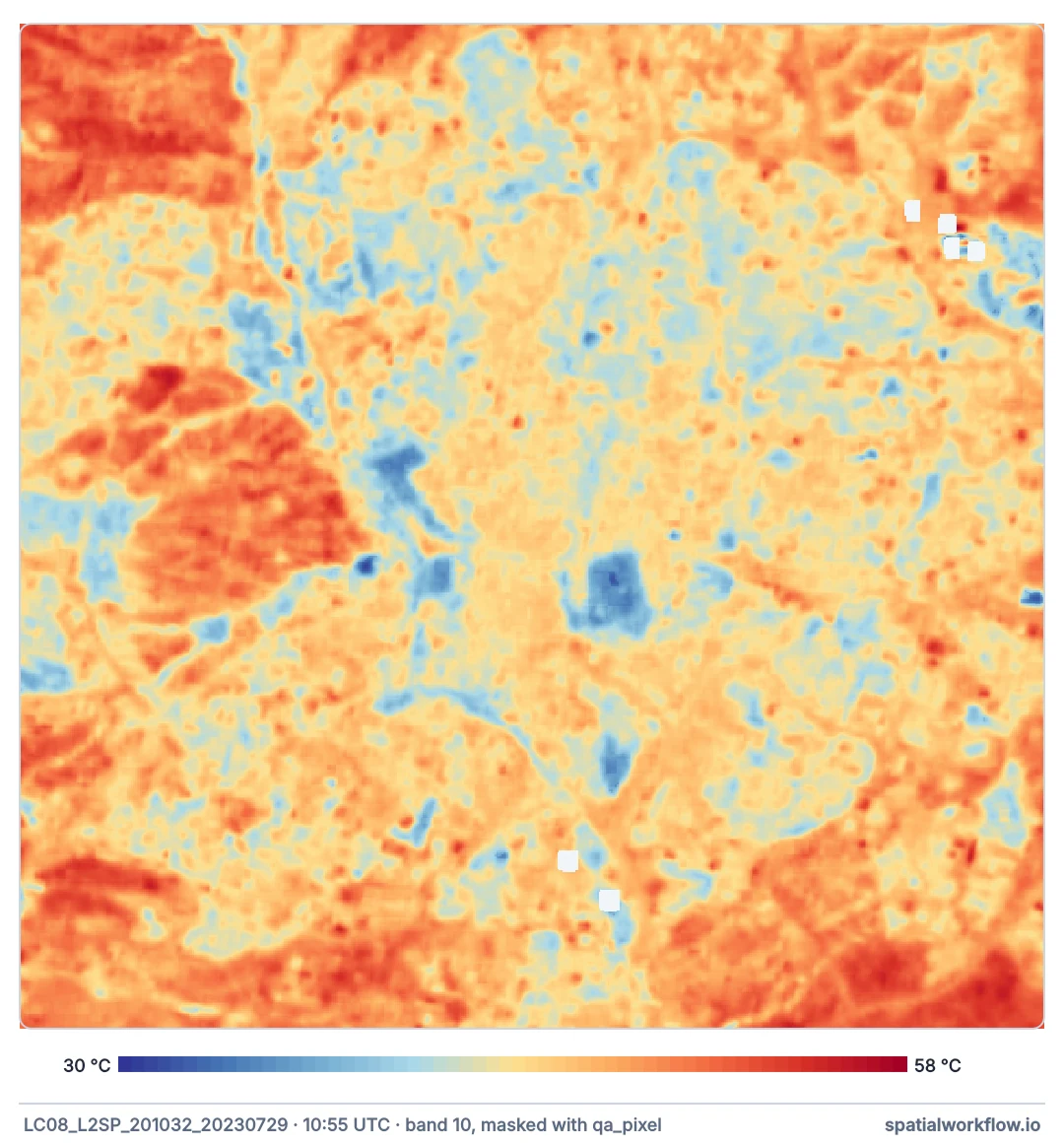
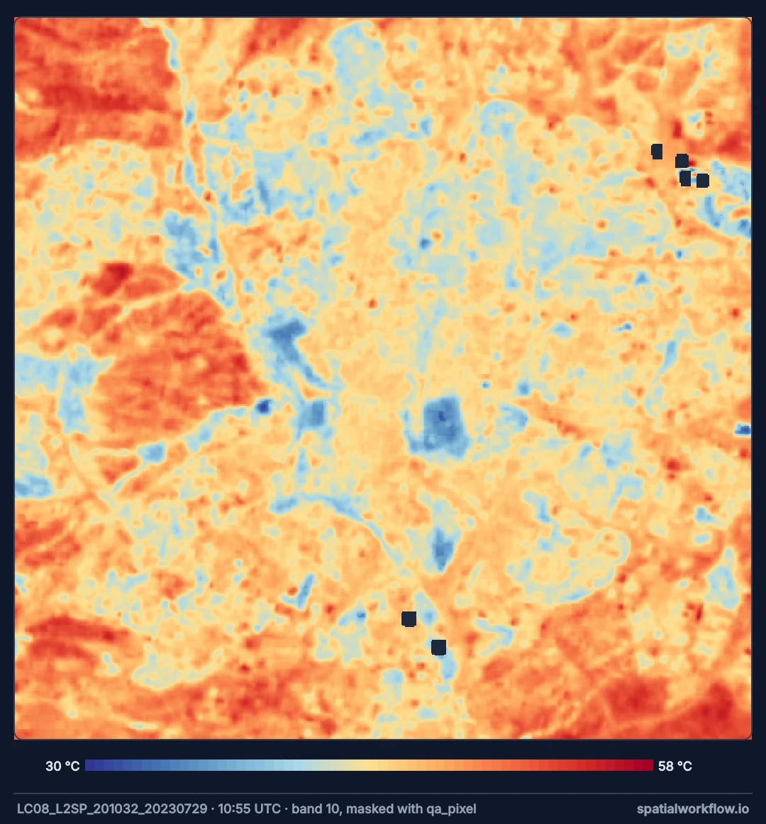
Right product, cloud filtering and masking, scale factors

1. Pick the right product and satellites

Collection 2 Level-2 (landsat-c2-l2) includes surface temperature. Landsat 8 and 9 carry band 10 (lwir11); Landsat 7 and 5 carry band 6 (lwir). Mixing them needs asset names per platform.

2. Filter scenes by cloud cover — then mask anyway

Scene-level cloud cover is for the whole 185 km scene. A scene with 5% cloud can have all of it over your city. The per-pixel QA band decides.

3. Read only your window

The assets are cloud-optimised GeoTIFFs in UTM. Transform your bounds into the scene CRS and read a window.

4. Apply the scale and offset

Surface temperature = DN × 0.00341802 + 149.0, in Kelvin. Subtract 273.15 for °C. DN 0 is fill.

5. Decode the QA bits

qa_pixel is a bit field: bit 0 fill, bit 1 dilated cloud, bit 3 cloud, bit 4 cloud shadow, bit 5 snow, bit 7 water. Mask clouds, their dilated edges and shadows.

6. Remember the native resolution

The thermal band is acquired at 100 m and delivered resampled to 30 m. Features smaller than about 100 m are blurred.

QA bits, raw values and a clean GeoTIFF

Example 1 — the QA bits, counted

bits = {0: "fill", 1: "dilated cloud", 3: "cloud", 4: "cloud shadow", 5: "snow", 7: "water"}
for b, name in bits.items():
    print(f"bit {b} ({name}): {((qa >> b) & 1).mean():.2%} of pixels")

bit 0 (fill): 0.00% of pixels
bit 1 (dilated cloud): 0.09% of pixels
bit 3 (cloud): 0.02% of pixels
bit 4 (cloud shadow): 0.11% of pixels
bit 5 (snow): 0.00% of pixels
bit 7 (water): 0.11% of pixels

On a clear summer scene most bits are rare; the water bit catches reservoirs and rivers, which are the coolest surfaces in the city and worth keeping separate rather than masking.

Example 2 — what the raw numbers look like

print(f"raw DN: min {dn[dn > 0].min()}, max {dn.max()}, dtype {dn.dtype}")
print(f"× 0.00341802 + 149 = {dn[dn > 0].min() * 0.00341802 + 149:.1f} to "
      f"{dn.max() * 0.00341802 + 149:.1f} K")

raw DN: min 43015, max 53437, dtype uint16
× 0.00341802 + 149 = 296.0 to 331.6 K

Integers in the tens of thousands, Kelvin after scaling, Celsius after the offset. Every step is a place a factor can be lost.

Example 3 — save a clean GeoTIFF

profile = {"driver": "GTiff", "height": lst.shape[0], "width": lst.shape[1], "count": 1,
           "dtype": "float32", "crs": crs, "transform": tf, "nodata": np.nan, "compress": "deflate"}
with rasterio.open(f"madrid_lst_{item.datetime:%Y%m%d}.tif", "w", **profile) as dst:
    dst.write(lst.astype("float32"), 1)
    dst.update_tags(1, units="degC", source=item.id, masked="cloud, dilated cloud, shadow")
print("saved with units and provenance in the tags")

saved with units and provenance in the tags

Recording the unit, the scene and the masking in the file saves the next reader from guessing.

Hotter than the air, and stored as integers

Why surface temperature is so much hotter than the air

A dark roof or road in full sun absorbs most of the incoming radiation and heats until it sheds that energy by convection and radiation. At midday in summer its surface can be 20–30 °C above the air a few metres above it. Surface temperature measures that skin, not the air people breathe.

Why the scale factor exists

Storing temperatures as 16-bit integers with a scale and offset keeps files small while preserving about 0.003 K precision. The factors are published in the product guide and repeated in the STAC metadata; they are the same for every Collection 2 Level-2 scene.

Why the overpass time matters

Landsat 8 and 9 cross the equator at about 10:00–10:15 local solar time. That is late morning: surfaces are heating but have not peaked. Afternoon maxima are higher, and night-time heat islands — often the ones that matter most for health — are invisible to Landsat.

Landsat 7, water and tokens

• Landsat 7 has a drifted orbit and scan-line gaps after 2003; treat it separately.
• Emissivity is built into the Level-2 product; do not correct again.
• Water: the product is valid over water, but water temperatures behave differently; keep the water bit as a class.
• Tier 2 scenes have poorer geometric accuracy; prefer Tier 1 (_T1) for urban work.
• Planetary Computer tokens expire; sign assets at read time.

Internal links

• Land surface temperature explained — what the number is
• Landsat thermal data explained — bands, resolution and overpass
• LST values on the wrong scale — the fix guide for the integers
• How to build a summer LST composite — beyond one scene
• Clouds show up as cold spots — masking failures
• How to download satellite imagery from STAC — the catalogue

FAQ

How do I convert Landsat surface temperature to Celsius?

DN × 0.00341802 + 149.0 gives Kelvin; subtract 273.15 for °C. DN 0 is fill.

Which band is surface temperature?

In Collection 2 Level-2, ST_B10 for Landsat 8/9 (lwir11 on the Planetary Computer) and ST_B6 for Landsat 5/7 (lwir).

How do I mask clouds?

Decode qa_pixel: exclude bits 1 (dilated cloud), 3 (cloud) and 4 (cloud shadow).

What resolution is Landsat thermal data?

Acquired at 100 m (Landsat 8/9), delivered resampled to 30 m.

What time of day is Landsat LST?

Late morning, around 10:00–10:30 local solar time.

Is LST the same as air temperature?

No. It is the temperature of the surface, often much hotter than the air in daytime.