How to Build a Summer Land Surface Temperature Composite in Python

On this page

Problem statement

A single Landsat scene is one late morning. Its surface temperatures depend on that day's weather — how hot, how windy, how long since rain — as much as on the city. Heat maps meant to guide tree planting or cool-roof programmes should show where surfaces are persistently hot, which needs many clear scenes combined into one composite with a known number of observations per pixel.

The steps are standard: collect the summer's scenes, mask each one, put them all on one grid, take a per-pixel statistic (usually the median) and keep the count. The care is in the grid, the masking and in not mixing sensors or times of day that are not comparable.

Quick answer

import numpy as np, rasterio, pystac_client, planetary_computer
from rasterio.warp import reproject, Resampling, transform_bounds
from rasterio.transform import from_origin

AOI = (-4.05, 40.20, -3.35, 40.65)                    # Madrid and its rural surroundings
DST_CRS = "EPSG:32630"                                           # UTM 30N, Landsat's own zone here
x0, y0, x1, y1 = transform_bounds("EPSG:4326", DST_CRS, *AOI)
x0, y1 = np.floor(x0 / 30) * 30, np.ceil(y1 / 30) * 30
W, H = int(np.ceil((x1 - x0) / 30)), int(np.ceil((y1 - y0) / 30))
DST_TF = from_origin(x0, y1, 30, 30)

cat = pystac_client.Client.open("https://planetarycomputer.microsoft.com/api/stac/v1")
items = [i for i in cat.search(collections=["landsat-c2-l2"], bbox=list(AOI),
                               datetime="2023-06-01/2023-08-31").items()
         if i.properties["platform"] in ("landsat-8", "landsat-9")
         and i.properties["eo:cloud_cover"] < 60]

def on_grid(item, asset, resampling=Resampling.nearest):
    out = np.zeros((H, W), dtype="uint16")
    with rasterio.open(planetary_computer.sign(item.assets[asset].href)) as src:
        reproject(rasterio.band(src, 1), out, dst_transform=DST_TF, dst_crs=DST_CRS,
                  resampling=resampling, src_nodata=0 if asset == "lwir11" else 1, dst_nodata=0)
    return out

layers = []
for it in sorted(items, key=lambda i: i.datetime):
    dn = on_grid(it, "lwir11")
    qa = on_grid(it, "qa_pixel")
    t = np.where(dn == 0, np.nan, dn * 0.00341802 + 149.0 - 273.15)
    bad = ((qa >> 1) & 1) | ((qa >> 3) & 1) | ((qa >> 4) & 1)
    t[bad == 1] = np.nan
    clear = np.isfinite(t).mean()
    print(f"{it.datetime:%Y-%m-%d} {it.properties['platform']}: {clear:5.0%} clear, "
          f"median {np.nanmedian(t) if clear else float('nan'):5.1f} °C")
    if clear > 0.2:
        layers.append(t)

stack = np.stack(layers)
median = np.nanmedian(stack, axis=0)
count = np.isfinite(stack).sum(axis=0)
print(f"\n{len(layers)} usable scenes; clear observations per pixel: "
      f"min {count.min()}, median {np.median(count):.0f}")
print(f"composite median LST: {np.nanmedian(median):.1f} °C, "
      f"5th–95th percentile {np.nanpercentile(median, 5):.1f}–{np.nanpercentile(median, 95):.1f} °C")

2023-06-03 landsat-9:   72% clear, median  33.2 °C
2023-06-04 landsat-8:    1% clear, median  33.0 °C
2023-06-11 landsat-8:   62% clear, median  39.3 °C
2023-06-12 landsat-9:    5% clear, median  36.8 °C
2023-06-19 landsat-9:   64% clear, median  36.9 °C
2023-06-20 landsat-8:    2% clear, median  35.0 °C
2023-06-27 landsat-8:  100% clear, median  44.9 °C
2023-06-28 landsat-9:    4% clear, median  48.5 °C
2023-07-05 landsat-9:   71% clear, median  46.0 °C
2023-07-06 landsat-8:    3% clear, median  47.6 °C
2023-07-13 landsat-8:  100% clear, median  50.1 °C
2023-07-14 landsat-9:    5% clear, median  48.3 °C
2023-07-21 landsat-9:   67% clear, median  47.0 °C
2023-07-22 landsat-8:    0% clear, median  37.4 °C
2023-07-29 landsat-8:  100% clear, median  48.8 °C
2023-07-30 landsat-9:    3% clear, median  50.5 °C
2023-08-06 landsat-9:  100% clear, median  48.4 °C
2023-08-07 landsat-8:    3% clear, median  49.2 °C
2023-08-14 landsat-8:  100% clear, median  46.9 °C
2023-08-15 landsat-9:    3% clear, median  48.2 °C
2023-08-22 landsat-9:  100% clear, median  51.2 °C
2023-08-23 landsat-8:    4% clear, median  52.1 °C
2023-08-30 landsat-8:   95% clear, median  40.6 °C

12 usable scenes; clear observations per pixel: min 0, median 10
composite median LST: 46.9 °C, 5th–95th percentile 40.6–51.3 °C

Scenes alternate between two neighbouring Landsat paths, a day apart. The ones with 0–5% "clear" are not cloudy: their path only clips the edge of the area, and the rest of the window is outside the swath. Of the scenes that cover it, most are entirely clear — it was a dry summer — and still their medians run from 33 °C in early June to 51 °C in late August. That day-to-day range is the reason a composite is needed.

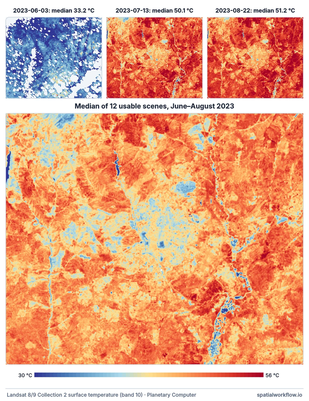
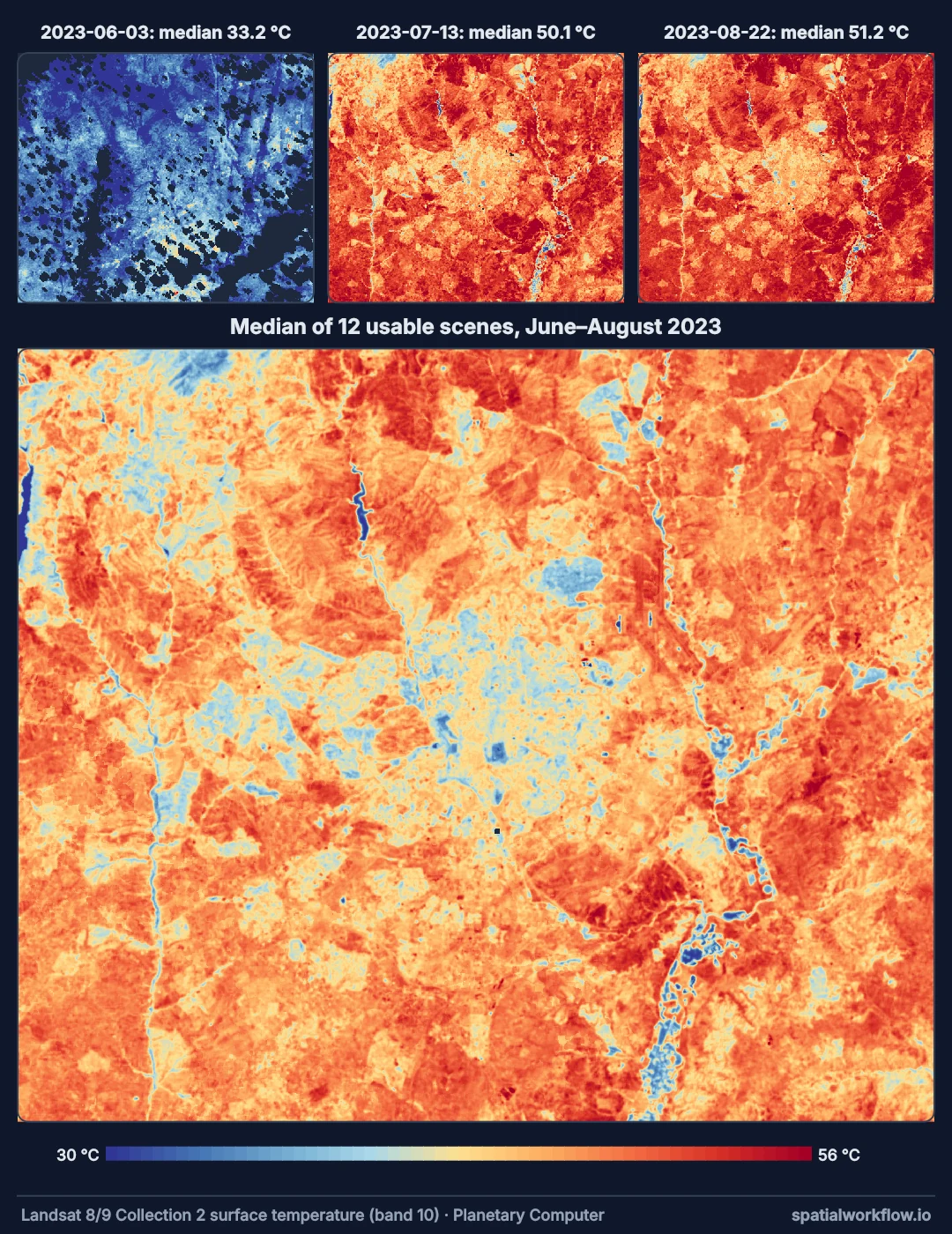
Three single-day land surface temperature maps of the Madrid area above one larger composite map, all on the same colour scale. The early June day is much cooler and patchy with gaps; the July and August days are hot; the composite is a complete summer picture. — Three of the twelve usable days and the composite, on one colour scale. 3 June is 18 °C cooler than 22 August at the median and has gaps where the scene was masked; any single day is a statement about that day. The median of all twelve is a complete picture of the summer: the reservoirs and river valleys cool, the dry farmland to the east and south hottest, the city in between.

One sensor, one grid, masked scenes, a median

1. Choose one sensor family and one time of day

Landsat 8 and 9 overpass at the same local time and share band design. Landsat 7's orbit has drifted to an earlier time; mixing it in adds scenes from a cooler part of the morning.

2. Define the output grid once

Snap the origin to the 30 m Landsat grid in the scene's UTM zone and reproject every scene onto it with nearest-neighbour resampling. That keeps pixels aligned across scenes from different paths.

3. Mask each scene before stacking

Clouds, dilated cloud edges and shadows per scene. A composite of unmasked scenes has cold holes wherever a cloud once sat.

4. Take the median, keep the count

The median resists residual cloud and haze better than the mean. The count of clear observations per pixel is part of the result.

5. Consider normalising for the day

Scenes on hotter days lift every pixel. Subtracting each scene's median (a relative anomaly) before compositing maps where the city is hot relative to itself, independent of which days were clear.

Many late mornings, one map, with the evidence count beside it.

Absolute against relative composites

Example 1 — absolute against relative composites

anomalies = np.stack([t - np.nanmedian(t) for t in layers])
rel = np.nanmedian(anomalies, axis=0)
day_medians = [np.nanmedian(t) for t in layers]
print(f"scene medians ranged {min(day_medians):.1f}–{max(day_medians):.1f} °C across the summer")
print(f"relative composite: coolest 5% at {np.nanpercentile(rel, 5):+.1f} °C, "
      f"hottest 5% at {np.nanpercentile(rel, 95):+.1f} °C relative to each scene's median")

scene medians ranged 33.2–51.2 °C across the summer
relative composite: coolest 5% at -6.5 °C, hottest 5% at +4.4 °C relative to each scene's median

The relative composite removes the day-to-day swing and keeps the pattern: which parts of the city are consistently hotter or cooler than the city as a whole.

Example 2 — how stable is the pattern?

from itertools import combinations
flat = [a[np.isfinite(a)] for a in anomalies]
mask = np.all(np.isfinite(anomalies), axis=0)
pairs = [np.corrcoef(anomalies[i][mask], anomalies[j][mask])[0, 1]
         for i, j in combinations(range(len(layers)), 2)]
print(f"pixels clear in every scene: {mask.mean():.0%}")
print(f"correlation of the spatial pattern between scenes: median {np.median(pairs):.2f}, "
      f"range {min(pairs):.2f}–{max(pairs):.2f}")

pixels clear in every scene: 13%
correlation of the spatial pattern between scenes: median 0.56, range 0.13–0.98

The median correlation between two scenes' spatial patterns is 0.56, and the most similar pairs reach 0.98. The hot and cool places largely repeat from one clear day to the next — the pattern is mostly a property of the city's surfaces — but any single scene is a noisy sample of it, which is what a composite averages away. Only 13% of pixels are clear in every scene, so the count band matters.

Example 3 — save value and count

profile = {"driver": "GTiff", "height": H, "width": W, "count": 2, "dtype": "float32",
           "crs": DST_CRS, "transform": DST_TF, "nodata": np.nan, "compress": "deflate"}
with rasterio.open("madrid_lst_jja2023.tif", "w", **profile) as dst:
    dst.write(median.astype("float32"), 1)
    dst.write(count.astype("float32"), 2)
    dst.set_band_description(1, "median LST °C, Landsat 8/9, Jun–Aug 2023")
    dst.set_band_description(2, "clear observations")
print(f"saved {W} × {H} composite")

saved 1994 × 1682 composite

The composite is the input for the heat-island, vegetation and neighbourhood guides.

The day matters: scene medians across one summer.

Why the median and relative values

Why the median

Residual cloud edges, thin cirrus and haze make pixels cooler than the true surface; occasional hot artefacts occur too. The median ignores both tails as long as they are a minority of a pixel's observations, which is why it is the default statistic for optical and thermal composites.

Why relative composites are useful

Absolute composites answer "how hot are these surfaces on typical clear summer mornings". Relative ones answer "where is the city hot compared with itself", which is less sensitive to which days happened to be clear and more comparable between years.

Why the grid matters

Landsat scenes from adjacent paths share the UTM grid in principle, but a window read from each scene can start at a different pixel. Reprojecting onto one snapped grid guarantees that pixel (i, j) is the same ground in every layer.

A composite without its evidence is a map of unknown days.

Two paths, heatwaves and minimum counts

Two paths can cover a city on different days; both are fine if they share the overpass time.
Heatwave vs typical: a composite of heatwave days only is a different product; say which.
Water pixels are cool and stable; mask them if the analysis is about land surfaces.
Minimum count: flag pixels with few clear observations; their median is noisy.
Memory: a summer of scenes over a city is small; a whole region needs chunked processing.

Internal links

How to read Landsat surface temperature — one scene, in detail
LST scenes are not comparable — the fix guide for mixing dates and sensors
How to calculate surface urban heat island intensity — the next step
Clouds show up as cold spots — masking before compositing
How to build a cloud-free Sentinel-2 composite — the same idea for reflectance
Landsat thermal data explained — sensors and overpass times

FAQ

How do I make a land surface temperature composite?

Mask each clear scene, reproject all to one grid, and take the per-pixel median of the clear observations, keeping a count.

Should I include Landsat 7?

Not with Landsat 8/9 in the same composite: its overpass time has drifted earlier and it has scan-line gaps.

Median or mean?

Median: it resists residual clouds and artefacts.

What is a relative LST composite?

A composite of each scene minus its own median, showing where the city is hotter or cooler than itself.

How many scenes do I need?

As many clear ones as the season offers; five or more per pixel gives a stable median.

Does the hot spot pattern change between days?

Usually little — scene-to-scene correlations of the spatial pattern are high on clear days.