How to Calculate Surface Urban Heat Island Intensity in Python

Problem statement

"The city is 4 °C hotter than its surroundings" is the headline number of every urban heat study, and it is built from three choices: what counts as urban, what counts as the surroundings, and which surface temperatures are compared. The surface urban heat island (SUHI) intensity — urban mean LST minus rural mean LST — can be positive, zero or negative for the same city depending on those choices, and in dry climates the daytime answer is often negative: irrigated parks and shaded streets can be cooler than sun-baked fields around the city.

Computing it well means defining urban and rural from data, excluding water and other surfaces that are neither, and reporting the definitions with the number.

Quick answer

Classify pixels as urban and rural from a built-up map, then compare median LST:

import numpy as np, rasterio, pystac_client, planetary_computer
from rasterio.warp import reproject, Resampling
from scipy import ndimage

with rasterio.open("madrid_lst_jja2023.tif") as src:              # from the composite guide
    lst, count = src.read(1), src.read(2)
    tf, crs, shape = src.transform, src.crs, (src.height, src.width)

cat = pystac_client.Client.open("https://planetarycomputer.microsoft.com/api/stac/v1")
wc_codes = np.zeros(shape, dtype="uint8")                       # WorldCover class on the LST grid
for it in cat.search(collections=["esa-worldcover"], bbox=[-4.05, 40.20, -3.35, 40.65],
                     datetime="2021-01-01/2021-12-31").items():
    with rasterio.open(planetary_computer.sign(it.assets["map"].href)) as src:
        tmp = np.zeros(shape, dtype="uint8")
        reproject(rasterio.band(src, 1), tmp, dst_transform=tf, dst_crs=crs,
                  resampling=Resampling.mode)                    # majority of the 10 m classes
        wc_codes = np.where(wc_codes == 0, tmp, wc_codes)

urban = wc_codes == 50                                           # built-up
water = wc_codes == 80
core_labels, _ = ndimage.label(urban)
biggest = np.bincount(core_labels.ravel())[1:].argmax() + 1
city = ndimage.binary_closing(core_labels == biggest, iterations=10)   # the continuous city
dist_km = ndimage.distance_transform_edt(~city) * 30 / 1000
rural = (dist_km > 5) & (dist_km <= 15) & ~urban & ~water
valid = np.isfinite(lst) & (count >= 3)
u, r = np.nanmedian(lst[city & urban & valid]), np.nanmedian(lst[rural & valid])
print(f"urban pixels: {(city & urban & valid).sum():,}, rural reference: {(rural & valid).sum():,}")
print(f"median LST urban {u:.1f} °C, rural {r:.1f} °C → SUHI intensity {u - r:+.1f} °C")

urban pixels: 501,458, rural reference: 629,436
median LST urban 44.4 °C, rural 48.0 °C → SUHI intensity -3.6 °C

The sign of that number is the first thing to look at, and here it is negative: at late morning in summer 2023, Madrid's built-up surfaces are 3.6 °C cooler than the dry farmland and grassland around them. For a dry, sunny city by day that is normal.

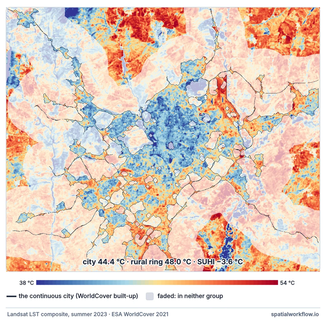
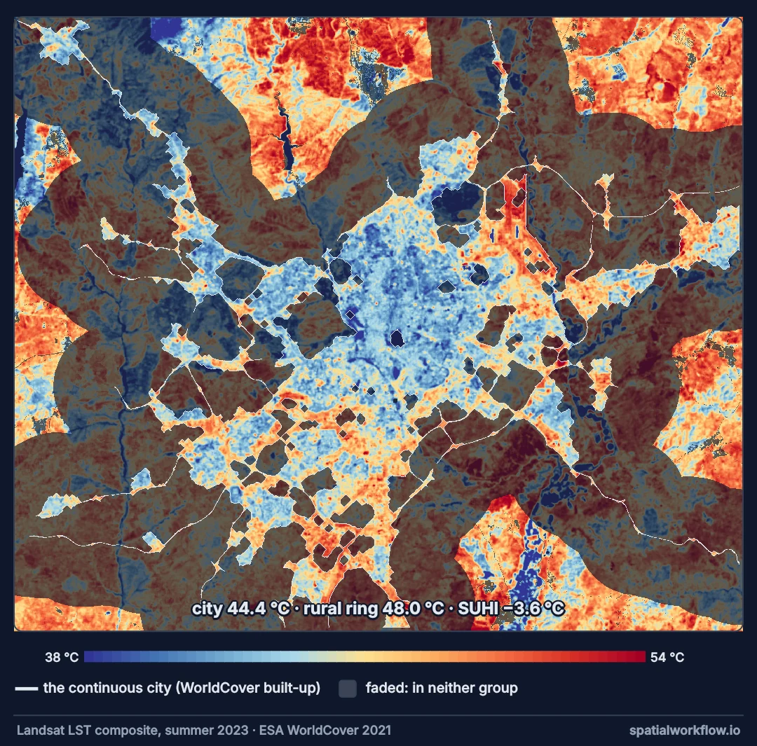
Urban from data, a rural ring, exclusions, medians

1. Define urban from data

A built-up class on a land cover map (here WorldCover's built-up class, taken as the majority of each 30 m pixel), restricted to the main continuous urban area. Administrative boundaries include too much non-urban land.

2. Define a rural reference ring

Land at a fixed distance from the urban edge (here 5–15 km), mostly unbuilt. The ring should be far enough to escape the city's influence and near enough to share its climate.

3. Exclude surfaces that are neither

Water is much cooler than anything else and belongs in neither group. Forest, irrigated farmland and bare ground in the ring all change the reference and should be reported.

4. Compare medians of a composite

Use a multi-scene composite, not one day; use medians, not means, to limit the influence of leftovers.

5. Report the definitions and the time

The SUHI is a statement about late-morning summer surfaces with a particular urban and rural definition. Night-time and air-temperature heat islands are different quantities.

What the rural ring is made of

The data used on this page

The summer 2023 land surface temperature composite of Madrid from the composite guide: the median of every Landsat 8 and 9 Collection 2 Level-2 scene from June to August 2023 on the Microsoft Planetary Computer with more than a fifth of the area clear, on a 30 m UTM 30N grid, with the count of clear observations as a second band. The setup rebuilds it if madrid_lst_jja2023.tif is missing.

import os

import numpy as np
import planetary_computer
import pystac_client
import rasterio
from rasterio.transform import from_origin
from rasterio.warp import Resampling, reproject, transform_bounds

if not os.path.exists("madrid_lst_jja2023.tif"):        # the composite guide's code, without the prints
    AOI = (-4.05, 40.20, -3.35, 40.65)
    DST_CRS = "EPSG:32630"
    x0, y0, x1, y1 = transform_bounds("EPSG:4326", DST_CRS, *AOI)
    x0, y1 = np.floor(x0 / 30) * 30, np.ceil(y1 / 30) * 30
    W, H = int(np.ceil((x1 - x0) / 30)), int(np.ceil((y1 - y0) / 30))
    DST_TF = from_origin(x0, y1, 30, 30)
    cat = pystac_client.Client.open("https://planetarycomputer.microsoft.com/api/stac/v1")
    items = [i for i in cat.search(collections=["landsat-c2-l2"], bbox=list(AOI),
                                   datetime="2023-06-01/2023-08-31").items()
             if i.properties["platform"] in ("landsat-8", "landsat-9") and i.properties["eo:cloud_cover"] < 60]

    def on_grid(item, asset):
        out = np.zeros((H, W), dtype="uint16")
        with rasterio.open(planetary_computer.sign(item.assets[asset].href)) as src:
            reproject(rasterio.band(src, 1), out, dst_transform=DST_TF, dst_crs=DST_CRS,
                      resampling=Resampling.nearest, src_nodata=0 if asset == "lwir11" else 1, dst_nodata=0)
        return out

    layers = []
    for it in sorted(items, key=lambda i: i.datetime):
        dn, qa = on_grid(it, "lwir11"), on_grid(it, "qa_pixel")
        t = np.where(dn == 0, np.nan, dn * 0.00341802 + 149.0 - 273.15)
        t[(((qa >> 1) & 1) | ((qa >> 3) & 1) | ((qa >> 4) & 1)) == 1] = np.nan
        if np.isfinite(t).mean() > 0.2:
            layers.append(t)
    stack = np.stack(layers)
    profile = {"driver": "GTiff", "height": H, "width": W, "count": 2, "dtype": "float32",
               "crs": DST_CRS, "transform": DST_TF, "nodata": np.nan, "compress": "deflate"}
    with rasterio.open("madrid_lst_jja2023.tif", "w", **profile) as dst:
        dst.write(np.nanmedian(stack, axis=0).astype("float32"), 1)
        dst.write(np.isfinite(stack).sum(axis=0).astype("float32"), 2)
        dst.set_band_description(1, "median LST °C, Landsat 8/9, Jun–Aug 2023")
        dst.set_band_description(2, "clear observations")
with rasterio.open("madrid_lst_jja2023.tif") as src:
    print(src.shape, src.crs, src.descriptions or "", f"median {np.nanmedian(src.read(1)):.1f} °C")

(1682, 1994) EPSG:32630 ('median LST °C, Landsat 8/9, Jun–Aug 2023', 'clear observations') median 46.9 °C

Example 1 — what the rural ring is made of

names = {10: "tree cover", 20: "shrubland", 30: "grassland", 40: "cropland", 50: "built-up", 60: "bare"}
ring = rural & valid
for code, name in names.items():
    m = ring & (wc_codes == code)
    if m.sum() > 1000:
        print(f"{name:<11} {m.sum() / ring.sum():5.1%} of the ring, median LST {np.nanmedian(lst[m]):5.1f} °C")

tree cover  16.3% of the ring, median LST  44.1 °C
shrubland    2.4% of the ring, median LST  44.6 °C
grassland   47.4% of the ring, median LST  48.6 °C
cropland    33.3% of the ring, median LST  48.8 °C
bare         0.6% of the ring, median LST  46.8 °C

The reference is a mix, and its classes differ in temperature by several degrees. A ring with more dry grassland makes the city look cooler; one with more forest makes it look hotter.

Example 2 — sensitivity to the ring distance

for lo, hi in ((2, 5), (5, 10), (5, 15), (10, 20), (15, 25)):
    ring_d = (dist_km > lo) & (dist_km <= hi) & ~urban & ~water & valid
    if ring_d.sum():
        print(f"ring {lo:>2}–{hi:<2} km: rural median {np.nanmedian(lst[ring_d]):5.1f} °C, "
              f"SUHI {u - np.nanmedian(lst[ring_d]):+5.1f} °C")

ring  2–5  km: rural median  47.7 °C, SUHI  -3.3 °C
ring  5–10 km: rural median  47.8 °C, SUHI  -3.4 °C
ring  5–15 km: rural median  48.0 °C, SUHI  -3.6 °C
ring 10–20 km: rural median  49.6 °C, SUHI  -5.2 °C

Moving the ring changes which landscapes form the reference — suburbs, farmland, the Sierra foothills — and the SUHI moves with it.

Example 3 — urban surfaces are not all hot

city_urban = city & urban & valid
green_in_city = city & (wc_codes == 10) & valid
print(f"built-up pixels in the city: median {np.nanmedian(lst[city_urban]):.1f} °C")
print(f"tree cover pixels in the city: median {np.nanmedian(lst[green_in_city]):.1f} °C "
      f"({green_in_city.sum():,} pixels)")
print(f"hottest 10% of city pixels above {np.nanpercentile(lst[city & valid], 90):.1f} °C")

built-up pixels in the city: median 44.4 °C
tree cover pixels in the city: median 42.2 °C (78,485 pixels)
hottest 10% of city pixels above 48.5 °C

Within the city, tree cover is 2.2 °C cooler than built-up land, and the hottest tenth of the city runs above 48.5 °C — hotter than the rural median. A single SUHI number averages that contrast away; the within-city spread is often more useful for planning.

Negative daytime islands and references

Why the SUHI can be negative in daytime

Surface temperature depends on how much absorbed sunlight is spent on evaporation. Dry summer fields have nothing to evaporate and heat strongly; cities have shade from buildings, irrigated parks and trees. In arid and Mediterranean climates the daytime surface heat island is weak or reversed; at night, when the city's stored heat is released, it reappears.

Why the reference defines the answer

The SUHI is a difference, so the rural mean matters as much as the urban one. There is no neutral countryside: it is farmland, forest, grassland or bare soil, each with its own temperature. Studies that compare cities with different surroundings compare their surroundings as much as their cities.

Why data-driven urban extents

Administrative boundaries of large cities include parks, forests and farmland; small municipalities split continuous cities. A built-up threshold follows the physical city and makes SUHI values comparable between places.

Elevation, coasts and seasons

• Elevation: rural references on higher ground are cooler for reasons unrelated to the city; restrict the ring's elevation range.
• Coastal cities need the sea excluded and often a one-sided ring.
• Seasons: winter SUHIs differ in sign and size from summer ones.
• Night-time LST (e.g. from ECOSTRESS or MODIS night passes) captures the heat island people feel at night.
• Air temperature heat islands are smaller than surface ones and peak at night.

Internal links

• Surface urban heat island explained — the concept in full
• SUHI rural reference wrong — the fix guide for the reference
• How to build a summer LST composite — the input
• How to relate LST to vegetation — why trees are cool
• Urban extent explained — defining the city
• How to compare land cover products for forest — WorldCover in detail

FAQ

How is surface urban heat island intensity calculated?

Median (or mean) LST of urban pixels minus that of a rural reference, from the same composite.

What is a good rural reference?

Mostly unbuilt land at a fixed distance from the urban edge, excluding water, at similar elevation.

Can the SUHI be negative?

Yes, in daytime in dry climates, where fields are hotter than shaded, irrigated urban areas.

Should I use administrative boundaries for "urban"?

No; use a built-up threshold on a land cover map for the continuous city.

Is the surface heat island the same as the air temperature heat island?

No. Surface differences are larger and peak in the day; air temperature differences are smaller and peak at night.

Why does my SUHI differ from published values?

Different urban and rural definitions, time of day, season, sensor and composite.