
How to Map Sentinel-5P NO2 in Python
On this page
Problem statement
Sentinel-5P's TROPOMI instrument maps nitrogen dioxide over the whole planet every day at a few kilometres' resolution, and the data is free. Turning it into a map of a city is still a small project. The Level-2 files are swaths, not grids: each pixel has its own latitude and longitude. A full-orbit file is 600 MB for the few hundred pixels that fall on London. Most pixels on most days are cloudy and must be discarded by a quality flag. And a monthly map is an average over whichever days happened to be clear, which has to be reported alongside it.
The workflow below reads only the pixels it needs, filters on quality, bins the swath onto a regular grid and keeps a count of how many observations went into each cell.
Quick answer
Search the Planetary Computer catalogue, keep daytime NO2 granules, read the variables lazily and filter on qa_value:
import numpy as np, pandas as pd, xarray as xr, fsspec
import pystac_client, planetary_computer

BBOX = (-0.6, 51.25, 0.35, 51.75)                     # Greater London and a margin
cat = pystac_client.Client.open("https://planetarycomputer.microsoft.com/api/stac/v1")
items = [i for i in cat.search(collections=["sentinel-5p-l2-netcdf"], bbox=list(BBOX),
                               datetime="2023-06-01/2023-08-31").items()
         if i.properties["s5p:product_name"] == "no2"          # the server ignores query filters
         and i.properties["s5p:processing_mode"] == "NRTI"     # one copy of each pass
         and 9 <= i.datetime.hour <= 15]                        # daylight overpasses only
print(f"{len(items)} daytime NO2 granules over London, June–August 2023")

fs = fsspec.filesystem("http")

def pixels(item):
    """The granule's pixels inside BBOX, read with HTTP range requests."""
    with fs.open(planetary_computer.sign(item.assets["no2"].href), block_size=4 * 2**20, cache_type="blockcache") as f:
        with xr.open_dataset(f, group="PRODUCT", engine="h5netcdf") as ds:   # closed each pass
            lat, lon = ds.latitude[0].values, ds.longitude[0].values
            inside = (lat > BBOX[1]) & (lat < BBOX[3]) & (lon > BBOX[0]) & (lon < BBOX[2])
            rows = np.where(inside.any(axis=1))[0]
            if len(rows) == 0:
                return None
            sl = slice(rows.min(), rows.max() + 1)
            m = inside[sl]
            return pd.DataFrame({
                "lat": lat[sl][m], "lon": lon[sl][m],
                "no2": ds.nitrogendioxide_tropospheric_column[0, sl].values[m],   # mol/m²
                "qa": ds.qa_value[0, sl].values[m],
                "time": item.datetime})

frames = [p for p in (pixels(i) for i in items) if p is not None]
px = pd.concat(frames, ignore_index=True)
good = px[px.qa >= 0.75]
print(f"{len(px):,} pixels read, {len(good):,} pass qa_value ≥ 0.75 ({len(good) / len(px):.0%})")
print(f"mean tropospheric column over the clear pixels: {good.no2.mean() * 1e6:.1f} µmol/m²")
160 daytime NO2 granules over London, June–August 2023
15,957 pixels read, 4,980 pass qa_value ≥ 0.75 (31%)
mean tropospheric column over the clear pixels: 64.9 µmol/m²
Range requests read only the rows that touch the box instead of the whole file. The quality filter throws most of it away — which is normal for a cloudy maritime city, and the reason the number of observations per cell matters as much as the mean.
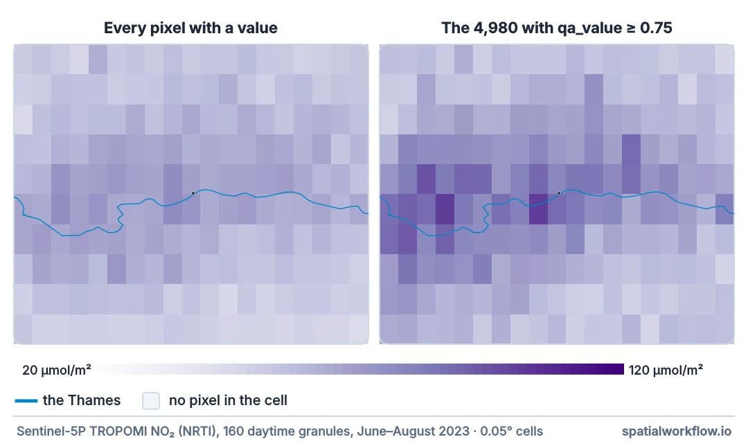
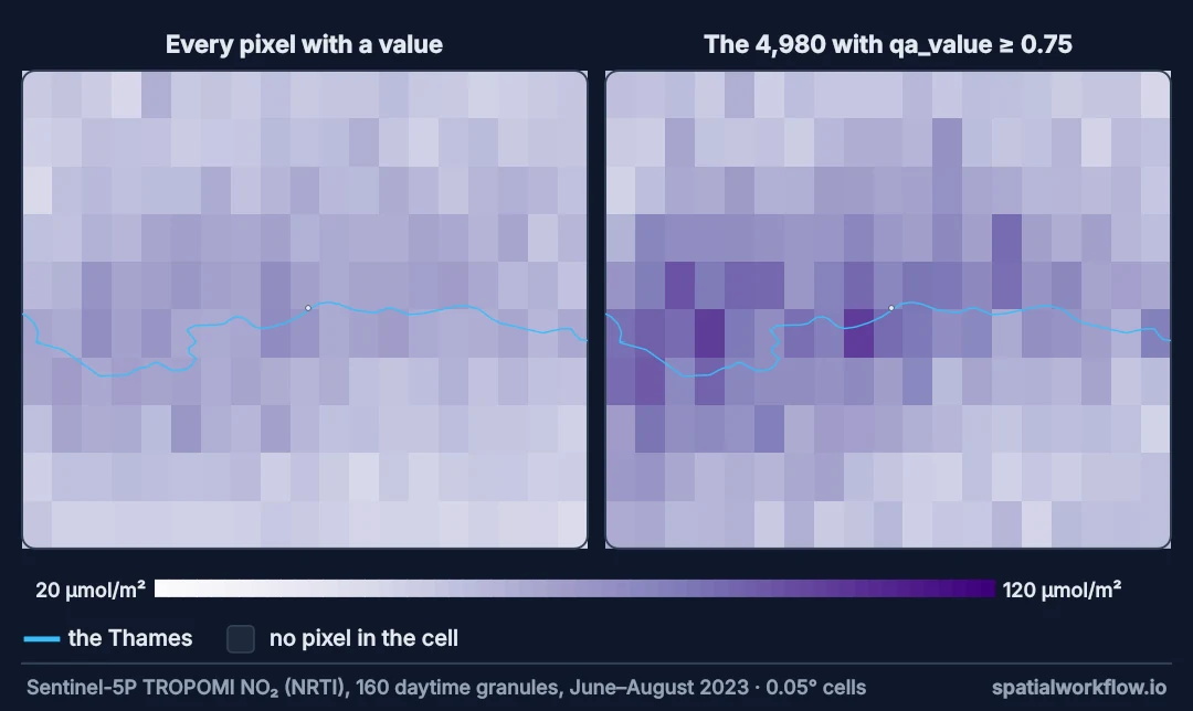
qa_value ≥ 0.75. The filtered map is higher — 64.9 against 58.3 µmol/m² on average — and it is the one where central London stands out along the Thames. Most of the unfiltered map is exactly the low-quality retrievals the flag exists to remove.Filter the catalogue, one stream, day passes, quality flags
1. Filter the catalogue yourself
The Planetary Computer STAC API returns every Sentinel-5P product intersecting the box — ozone, methane, clouds, aerosols — and ignores query filters. Filter on s5p:product_name and s5p:processing_mode client-side.
2. Keep one processing stream
Each pass exists as a near-real-time (NRTI) granule and, days later, inside an offline (OFFL) full-orbit file. Mixing them double-counts every day. OFFL is the reprocessed product for long-term science; NRTI granules are five-minute slices, far smaller to read, and fine for maps like this one.
3. Drop the night-side passes
Descending passes over the night side intersect the box but carry no NO2 retrieval — it needs sunlight. They appear in the search results; skip them by overpass hour.
4. Read only the rows you need
Read latitude and longitude, find the scanlines that touch the box, then read NO2 and qa_value for those rows only.
5. Filter on quality
qa_value ≥ 0.75 is the recommendation for most uses: it removes cloudy, snow-covered and problematic retrievals. Lower thresholds keep more pixels and more bias.
6. Bin onto a grid with counts
Assign each pixel centre to a regular grid cell and average. Keep the count per cell: a cell mean from three clear days is not comparable with one from forty.
From swaths to a gridded GeoTIFF over London
Example 1 — from swath to grid
res = 0.05                                                    # degrees, about 3.5 × 5.5 km here
good = good.assign(ix=((good.lon - BBOX[0]) // res).astype(int),
                   iy=((good.lat - BBOX[1]) // res).astype(int))
cells = good.groupby(["iy", "ix"]).agg(no2=("no2", "mean"), n=("no2", "size")).reset_index()
cells["no2_umol"] = cells.no2 * 1e6
print(f"{len(cells)} cells; observations per cell: median {cells.n.median():.0f}, "
      f"min {cells.n.min()}, max {cells.n.max()}")
top = cells.nlargest(3, "no2_umol")
for _, c in top.iterrows():
    print(f"  cell centred {BBOX[1] + (c.iy + .5) * res:.3f}°N {BBOX[0] + (c.ix + .5) * res:+.3f}°E: "
          f"{c.no2_umol:.0f} µmol/m² from {c.n:.0f} pixels")
190 cells; observations per cell: median 26, min 14, max 41
cell centred 51.475°N -0.175°E: 101 µmol/m² from 14 pixels
cell centred 51.475°N -0.425°E: 101 µmol/m² from 20 pixels
cell centred 51.525°N -0.475°E: 94 µmol/m² from 22 pixels
The top cells are south-west central London and, next to it, the cell over Heathrow airport and the M4/M25 junction — plausible sources, each resting on 14–22 clear pixels. Binning pixel centres is the simplest regridding and adequate when cells are similar in size to pixels. For finer grids, area-weighted regridding using the pixel corner coordinates avoids the checkerboard of empty cells.
Example 2 — write a GeoTIFF with the counts
import rasterio
from rasterio.transform import from_origin

nx = int(np.ceil((BBOX[2] - BBOX[0]) / res))
ny = int(np.ceil((BBOX[3] - BBOX[1]) / res))
mean = np.full((ny, nx), np.nan, dtype="float32")
count = np.zeros((ny, nx), dtype="uint16")
mean[ny - 1 - cells.iy, cells.ix] = cells.no2_umol
count[ny - 1 - cells.iy, cells.ix] = cells.n
with rasterio.open("london_no2_jja2023.tif", "w", driver="GTiff", width=nx, height=ny, count=2,
                   dtype="float32", crs="EPSG:4326", nodata=np.nan,
                   transform=from_origin(BBOX[0], BBOX[3], res, res)) as dst:
    dst.write(mean, 1)
    dst.write(count.astype("float32"), 2)
    dst.set_band_description(1, "tropospheric NO2, µmol/m², mean of qa>=0.75 pixels")
    dst.set_band_description(2, "number of pixels averaged")
print(f"wrote {nx} × {ny} cells, {np.isfinite(mean).mean():.0%} with data")
wrote 19 × 10 cells, 100% with data
Two bands, value and count, in one file: anybody using the map can see how much evidence is behind each cell.
Example 3 — the centre against the edge
centre = good[np.hypot(good.lat - 51.51, (good.lon + 0.12) * 0.62) < 0.08]
edge = good[np.hypot(good.lat - 51.51, (good.lon + 0.12) * 0.62) > 0.30]
print(f"central London (≈9 km radius): {centre.no2.mean() * 1e6:.0f} µmol/m² from {len(centre)} pixels")
print(f"outer ring (> 33 km):          {edge.no2.mean() * 1e6:.0f} µmol/m² from {len(edge)} pixels")
print(f"ratio {centre.no2.mean() / edge.no2.mean():.1f}")
central London (≈9 km radius): 80 µmol/m² from 312 pixels
outer ring (> 33 km): 58 µmol/m² from 589 pixels
ratio 1.4
The city stands out against its surroundings in a summer average, 1.4 times the outer ring. That contrast — the urban NO2 dome — is what satellite NO2 maps reliably; the difference between two streets is not.
Swaths, quality flags and two processing streams
Why the files are swaths
TROPOMI scans a 2,600 km-wide strip perpendicular to its track, 450 pixels across. The Level-2 product keeps that geometry, with a latitude and longitude for every pixel, because regridding loses information and every user wants a different grid. Pixels are about 5.5 × 3.5 km at nadir and larger towards the swath edges.
Why the quality flag removes so much
The retrieval needs to know how much of the light path was in the lower atmosphere. Clouds hide the boundary layer, where most NO2 is; snow and bright surfaces confuse the air-mass factor. qa_value folds all of that into one number, and 0.75 is the threshold below which the column is too uncertain for most uses.
Why NRTI and OFFL both appear
Near-real-time data is produced within hours for forecasting; offline data is reprocessed later with better inputs. The catalogue keeps both. For a map of a past period OFFL is preferable in principle; NRTI is much cheaper to read because each granule is five minutes of orbit rather than a full one, and the difference for a seasonal city map is small.
Units, pixel corners and SAS tokens
- Units:
mol/m²; multiply by 6.022 × 10¹⁹ for molecules/cm², the unit much of the literature uses. - Pixel corners (
latitude_bounds,longitude_boundsin the SUPPORT_DATA group) allow area-weighted regridding. - Processor versions change over time; long time series should use a consistently reprocessed product.
- Winter has fewer valid pixels at high latitudes because of low sun and snow.
- Planetary Computer SAS tokens expire; re-sign items if a long job starts failing with 403 errors.
Internal links
- Satellite NO2 explained — what a column is and what it is not
- Satellite NO2 map mostly empty — the fix guide for sparse maps
- How to download satellite imagery from STAC — the catalogue side
- How to open NetCDF with xarray — groups and variables
- How to calculate population-weighted exposure — combining a pollution grid with people
- Air pollutants and their units explained — surface concentrations, for contrast
FAQ
Where can I download Sentinel-5P NO2 data?
From the Copernicus Data Space, or through STAC catalogues such as Microsoft's Planetary Computer (sentinel-5p-l2-netcdf).
Which qa_value threshold should I use?
0.75 for most analyses of tropospheric NO2. Lower thresholds admit cloudy and snow-affected retrievals.
What is the difference between NRTI and OFFL?
NRTI is produced within hours in five-minute granules; OFFL is reprocessed later as full orbits. Use one, not both.
Why are there night-time granules in my search?
They intersect the area on the night side of the orbit. NO2 is not retrieved there; skip them.
How do I put the swath on a grid?
Bin pixel centres into grid cells and average, keeping a count per cell; or regrid area-weighted using the pixel corners.
What resolution is Sentinel-5P NO2?
About 5.5 × 3.5 km at nadir since August 2019, coarser towards the edges of the swath.