How to Compare Land Cover Products for Forest in Python

On this page

Problem statement

How much forest is there in this landscape? Three widely used global products give three answers: Hansen's tree cover (thresholded at a canopy percentage), ESA WorldCover's "tree cover" class, and Impact Observatory's annual land-use/land-cover "trees" class. They differ in year, resolution, classification method and — above all — definition. Choosing one without comparing it to the others hides a spread that can be larger than the change being measured.

The comparison needs the products on one grid, for the same year as nearly as possible, and an agreement table that shows where they disagree, not just how much.

Quick answer

Read each product for the same window, resample to one grid, and cross-tabulate:

import numpy as np, pandas as pd, rasterio
from rasterio.windows import from_bounds
from rasterio.warp import reproject, Resampling
import pystac_client, planetary_computer

W, S, E, N = -63.0, -10.8, -62.5, -10.3
with rasterio.open("rondonia_gfc.tif") as src:                  # Hansen stack, reading guide
    treecover, lossyear, datamask = src.read()
    tf, crs, shape = src.transform, src.crs, (src.height, src.width)
hansen = (treecover > 30) & ((lossyear == 0) | (lossyear > 21)) & (datamask == 1)   # forest in 2021

cat = pystac_client.Client.open("https://planetarycomputer.microsoft.com/api/stac/v1")
def on_grid(collection, dt, value_map):
    items = cat.search(collections=[collection], bbox=[W, S, E, N], datetime=dt).item_collection()
    out = np.zeros(shape, dtype="uint8")
    for it in items:
        href = planetary_computer.sign(it.assets["map" if "map" in it.assets else "data"].href)
        with rasterio.open(href) as src:
            tmp = np.zeros(shape, dtype="uint8")
            reproject(rasterio.band(src, 1), tmp, dst_transform=tf, dst_crs=crs,
                      resampling=Resampling.mode)
        out = np.where(out == 0, tmp, out)
    return np.isin(out, value_map), out

worldcover, wc_raw = on_grid("esa-worldcover", "2021-01-01/2021-12-31", [10])   # 10 = tree cover
iolulc, io_raw = on_grid("io-lulc-annual-v02", "2021-01-01/2021-12-31", [2])    # 2 = trees

px_ha = (abs(tf.a) * 111_320 * np.cos(np.radians((S + N) / 2))) * (abs(tf.e) * 110_574) / 1e4
for name, m in (("Hansen >30% canopy, 2021", hansen), ("ESA WorldCover 2021", worldcover),
                ("Impact Observatory 2021", iolulc)):
    print(f"{name:<26} forest {m.sum() * px_ha:>9,.0f} ha ({m.mean():.1%} of the window)")

Hansen >30% canopy, 2021   forest    85,260 ha (28.2% of the window)
ESA WorldCover 2021        forest    98,104 ha (32.4% of the window)
Impact Observatory 2021    forest    71,729 ha (23.7% of the window)

Three products, one landscape, three forest areas. The spread is the first number to know before using any of them.

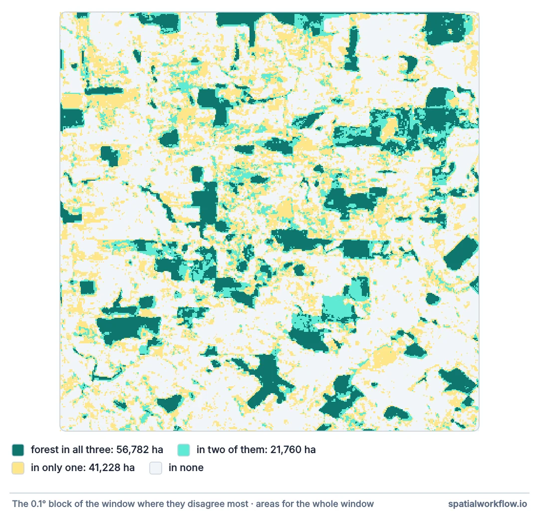
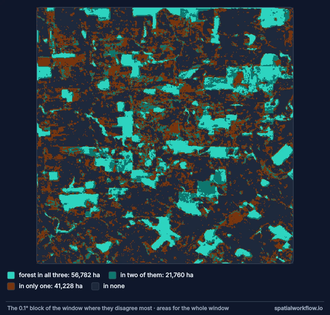
Close-up of Rondônia coloured by how many of three land-cover products call each pixel forest: solid blocks where all three agree, a fringe where two agree, and scattered yellow patches that only one product calls forest. — Where the three products agree, in the 0.1° block of the window where they disagree most. The solid forest blocks are forest in all three; the disagreement is at their edges and in the scattered regrowth between them. Across the whole window only 56,782 ha is forest in all three products, while 119,770 ha is forest in at least one — the whole spread between 71,729 and 98,104 ha lives in those fringes.

Align years, one grid, mapped definitions, cross-tabulate

1. Align the years

Hansen gives 2000 cover and annual loss, so forest in any later year is derived; WorldCover exists for 2020 and 2021; Impact Observatory is annual. Compare the same year.

2. Put everything on one grid

Resample categorical maps with the mode (majority), never bilinear. The coarsest native resolution is usually the honest common grid; here Hansen's 30 m.

3. Map each product's forest definition

WorldCover's tree cover class means ≥ 10% tree cover in a 10 m pixel; Impact Observatory's trees class is a learned label; Hansen needs an explicit canopy threshold. Write the mapping down.

4. Cross-tabulate

The agreement table — forest in both, in one only, in neither — shows where the products disagree, which is more informative than the totals.

5. Look at where they disagree

Disagreement concentrates at edges, in secondary regrowth, plantations and savanna. Those are often exactly the places an analysis cares about.

Three products, three definitions of a tree-covered pixel.

Where Hansen and WorldCover disagree

The data used on this page

A window over Rondônia, Brazil (63.0°–62.5°W, 10.8°–10.3°S): Hansen Global Forest Change v1.12 (tree cover in 2000, the year of loss, and the data mask) read from Google's storage into a three-band rondonia_gfc.tif, as in the Hansen reading guide; ESA WorldCover and Impact Observatory's annual land-use/land-cover map are read from the Microsoft Planetary Computer by the quick answer.

import os

import rasterio
from rasterio.windows import from_bounds

W, S, E, N = -63.0, -10.8, -62.5, -10.3
V = "GFC-2024-v1.12"
if not os.path.exists("rondonia_gfc.tif"):
    bands = []
    for name in ("treecover2000", "lossyear", "datamask"):
        url = f"https://storage.googleapis.com/earthenginepartners-hansen/{V}/Hansen_{V}_{name}_10S_070W.tif"
        with rasterio.open(url) as src:
            window = from_bounds(W, S, E, N, src.transform)
            bands.append(src.read(1, window=window))
            profile = src.profile | {"count": 3, "width": bands[0].shape[1], "height": bands[0].shape[0],
                                     "transform": src.window_transform(window), "compress": "deflate",
                                     "driver": "GTiff", "tiled": False}
    profile.pop("blockxsize", None)
    profile.pop("blockysize", None)
    with rasterio.open("rondonia_gfc.tif", "w", **profile) as dst:
        for i, band in enumerate(bands, start=1):
            dst.write(band, i)
with rasterio.open("rondonia_gfc.tif") as src:
    print(src.count, src.shape, src.crs, src.res)

3 (2000, 2000) EPSG:4326 (0.00025, 0.00025)

Example 1 — the agreement table

def agree(a, b, na, nb):
    t = pd.crosstab(pd.Series(a.ravel(), name=na), pd.Series(b.ravel(), name=nb), normalize=True)
    return (t * 100).round(1)
print(agree(hansen, worldcover, "Hansen", "WorldCover").to_string())
print()
print(agree(worldcover, iolulc, "WorldCover", "Impact Obs.").to_string())
all3 = hansen & worldcover & iolulc
any1 = hansen | worldcover | iolulc
print(f"\nforest in all three: {all3.mean():.1%} of the window; in at least one: {any1.mean():.1%}")

WorldCover  False  True 
Hansen                  
False        60.6   11.2
True          6.9   21.3

Impact Obs.  False  True 
WorldCover               
False         67.1    0.4
True           9.1   23.3

forest in all three: 18.8% of the window; in at least one: 39.6%

The core that all three call forest is smaller than any one product's forest; the band where at least one does is larger. The difference between them is the uncertainty in "how much forest is there".

Example 2 — where the disagreement sits

from scipy import ndimage
edge = ndimage.binary_dilation(all3, iterations=3) & ~ndimage.binary_erosion(all3, iterations=3)
disagree = any1 & ~all3
print(f"share of disagreement within ~90 m of the agreed forest edge: "
      f"{(disagree & edge).sum() / disagree.sum():.0%}")
cover_in_disagree = treecover[disagree]
print(f"Hansen 2000 canopy in disagreement pixels: median {np.median(cover_in_disagree):.0f}%")

share of disagreement within ~90 m of the agreed forest edge: 44%
Hansen 2000 canopy in disagreement pixels: median 59%

Nearly half of the disagreement lies within three pixels of the edge of the agreed forest and in pixels with intermediate canopy — the forest–pasture transition, where a 10 m and a 30 m classifier see different mixtures.

Example 3 — what WorldCover calls the Hansen forest

labels = {10: "tree cover", 20: "shrubland", 30: "grassland", 40: "cropland", 50: "built-up",
          60: "bare", 80: "water", 90: "herbaceous wetland"}
vals, counts = np.unique(wc_raw[hansen], return_counts=True)
for v, c in sorted(zip(vals, counts), key=lambda x: -x[1])[:5]:
    print(f"{labels.get(int(v), v):<18} {c / hansen.sum():.1%} of Hansen forest pixels")

tree cover         75.4% of Hansen forest pixels
grassland          24.4% of Hansen forest pixels
water              0.1% of Hansen forest pixels
built-up           0.0% of Hansen forest pixels
cropland           0.0% of Hansen forest pixels

Three-quarters of Hansen's forest pixels are tree cover in WorldCover too; nearly all the rest are grassland. These are pixels with enough canopy in 2000 and no recorded loss since that WorldCover's 2021 classifier nonetheless sees as grass — degraded forest, regrowth of an unrecorded clearing, or simply a different reading of a mixed pixel.

The forest all three agree on is smaller than any one of them.

Different questions, different resolutions

Why the products disagree

They answer different questions. Hansen maps canopy closure from Landsat time series; WorldCover and Impact Observatory classify Sentinel-2 imagery into land cover classes with different training data and class definitions. A pixel of young regrowth or a eucalyptus plantation can reasonably be "trees" in one and "grassland" or "cropland" in another.

Why resolution matters

A 10 m classifier separates a strip of trees along a stream from the pasture beside it; at 30 m the mixed pixel may fall either way. Resampling to a common grid with the mode keeps classes but decides each mixed pixel by majority, which is itself a source of disagreement.

Why agreement is not accuracy

Three products agreeing does not make a pixel correct; they share input imagery and similar methods. Accuracy needs independent reference data. Agreement is a cheap, useful indicator of where the uncertainty lies.

Four checks that make a product comparison fair.

Versions, classes and mode resampling

WorldCover versions: 2020 (v100) and 2021 (v200) used different algorithms; changes between them are not all real.
Impact Observatory classes changed between versions; check the class table for the collection used.
Planetary Computer signs asset URLs with expiring tokens; sign at read time for long jobs.
Mode resampling from 10 m to 30 m still leaves 3 × 3 ties possible; the result depends on the resampler.
Water masks differ between products too; mask with one of them consistently.

Internal links

Land cover products explained — the products and their definitions
Forest definitions explained — canopy thresholds and minimum areas
How to read Hansen Global Forest Change data — the Hansen stack
How to classify land cover in Python — making a map of your own
Raster resampling explained — mode against bilinear
How to download satellite imagery from STAC — the Planetary Computer side

FAQ

Which global land cover product is best for forest?

It depends on the definition and year you need. Compare them for your area before choosing.

Why do forest areas differ between products?

Different definitions, resolutions, years and classification methods.

How do I compare categorical rasters of different resolution?

Resample to a common grid with the mode (majority) and cross-tabulate.

Does agreement between products mean accuracy?

No. It indicates where uncertainty lies; accuracy needs independent reference data.

Where does disagreement usually occur?

At forest edges, in regrowth, plantations, shrubland and savanna.

Can I use WorldCover to measure change?

Not between its 2020 and 2021 versions, which used different algorithms.