Forest Area Wrong in Degrees

On this page

Problem statement

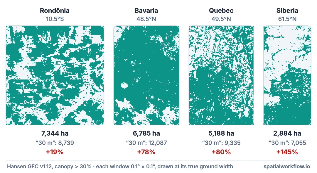
The forest area computed from the Hansen tiles comes out too high everywhere and badly too high in Canada or Siberia. The count of pixels is right; the conversion to hectares is not. The Global Forest Change layers are distributed on a geographic grid of 0.00025° — just under one arc-second — and a pixel is about 27.8 × 27.6 m at the equator and 13.9 × 27.6 m at 60°N. Multiplying every pixel by 0.09 ha — "30 m pixels" — overstates areas by about a sixth even at the equator, increasingly towards the poles, and differently for every row of a tile.

Quick answer

Compute each row's pixel area from its latitude, or reproject to an equal-area CRS before counting:

import numpy as np, rasterio
from rasterio.windows import from_bounds

def forest_area(tile, bounds, v="GFC-2024-v1.12", threshold=30):
    with rasterio.open(f"/vsicurl/https://storage.googleapis.com/earthenginepartners-hansen/"
                       f"{v}/Hansen_{v}_treecover2000_{tile}.tif") as src:
        win = from_bounds(*bounds, src.transform)
        tc = src.read(1, window=win)
        tf = src.window_transform(win)
    forest = tc > threshold
    naive_ha = forest.sum() * 0.09                                        # "30 m pixels"
    lat = bounds[3] - (np.arange(tc.shape[0]) + 0.5) * abs(tf.e)
    row_ha = (abs(tf.a) * 111_320 * np.cos(np.radians(lat))) * (abs(tf.e) * 110_574) / 1e4
    correct_ha = (forest.sum(axis=1) * row_ha).sum()
    return naive_ha, correct_ha

cases = {"Rondônia, 10.5°S": ("10S_070W", (-63.0, -10.6, -62.9, -10.5)),
         "Bavaria, 48.5°N": ("50N_010E", (13.3, 48.9, 13.4, 49.0)),
         "Quebec, 49.5°N": ("50N_080W", (-74.0, 49.4, -73.9, 49.5)),
         "Siberia, 61.5°N": ("70N_100E", (105.0, 61.4, 105.1, 61.5))}
print(f"{'place':<18}{'0.09 ha/pixel':>15}{'by latitude':>14}{'error':>8}")
for name, (tile, b) in cases.items():
    naive, correct = forest_area(tile, b)
    print(f"{name:<18}{naive:>15,.0f}{correct:>14,.0f}{naive / correct - 1:>8.0%}")

place               0.09 ha/pixel   by latitude   error
Rondônia, 10.5°S            8,739         7,344     19%
Bavaria, 48.5°N            12,087         6,785     78%
Quebec, 49.5°N              9,335         5,188     80%
Siberia, 61.5°N             7,055         2,884    145%

Even in Rondônia, 10° from the equator, the naive factor overstates the forest by 19%; at 48–50°N by about 80%; at 61.5°N it multiplies it by two and a half. The error is worst in exactly the boreal and temperate studies where it is least expected, because "30 m" sounds like a constant.

Four forest maps of the same size in degrees, drawn at their true ground width: Rondônia near the equator is almost square, Siberia at 61.5 degrees north is barely half as wide. Under each, the correct forest area, the naive area and the error. — Each window is 0.1° × 0.1°, the same number of pixels, and each is drawn here at its true width on the ground. A degree of longitude shrinks with the cosine of latitude, so the Siberian window is barely half as wide as the Rondônian one — and a flat 0.09 ha per pixel overstates its forest by 145%.

Recognise the grid, use row-wise areas or reproject

1. Recognise the grid

If the CRS is EPSG:4326 and the resolution is 0.00025°, pixels are not squares on the ground and not all the same size.

2. Use row-wise pixel areas for small areas

Pixel width shrinks with cos(latitude); pixel height is nearly constant. Compute the area of each row and weight counts by it.

3. Reproject to an equal-area CRS for large areas

For countries or continents, reproject the classified raster (nearest neighbour) to an equal-area projection and count pixels of known, constant area.

4. Never resample categories bilinearly

When reprojecting a forest mask or loss-year layer, use nearest neighbour or mode; bilinear invents intermediate values.

5. Check with a polygon

Compare your total for a region with the region's area computed in an equal-area CRS; the forest share must be at most 100%.

The same 0.00025°, narrower on the ground with every degree of latitude.

The error by latitude, and a guard

Example 1 — the error by latitude

for lat in (0, 10, 30, 45, 50, 60, 70):
    w_m = 0.00025 * 111_320 * np.cos(np.radians(lat))             # the GFC grid step
    h_m = 0.00025 * 110_574
    print(f"{lat:>2}°: pixel {w_m:4.1f} × {h_m:4.1f} m = {w_m * h_m / 1e4:.4f} ha; "
          f"0.09 ha overstates by {0.09 / (w_m * h_m / 1e4) - 1:5.0%}")

 0°: pixel 27.8 × 27.6 m = 0.0769 ha; 0.09 ha overstates by   17%
10°: pixel 27.4 × 27.6 m = 0.0758 ha; 0.09 ha overstates by   19%
30°: pixel 24.1 × 27.6 m = 0.0666 ha; 0.09 ha overstates by   35%
45°: pixel 19.7 × 27.6 m = 0.0544 ha; 0.09 ha overstates by   65%
50°: pixel 17.9 × 27.6 m = 0.0495 ha; 0.09 ha overstates by   82%
60°: pixel 13.9 × 27.6 m = 0.0385 ha; 0.09 ha overstates by  134%
70°: pixel  9.5 × 27.6 m = 0.0263 ha; 0.09 ha overstates by  242%

The error is systematic: it grows with latitude and never cancels. A global total built on 0.09 ha per pixel overweights boreal forest relative to tropical forest.

Example 2 — equal-area reprojection as a check

from rasterio.warp import reproject, Resampling, calculate_default_transform
tile, b = cases["Siberia, 61.5°N"]
with rasterio.open(f"/vsicurl/https://storage.googleapis.com/earthenginepartners-hansen/"
                   f"GFC-2024-v1.12/Hansen_GFC-2024-v1.12_treecover2000_{tile}.tif") as src:
    win = from_bounds(*b, src.transform)
    tc = src.read(1, window=win)
    tf = src.window_transform(win)
dst_crs = "EPSG:6933"                                                  # WGS 84 / NSIDC EASE-Grid 2.0, equal area
dtf, w, h = calculate_default_transform("EPSG:4326", dst_crs, tc.shape[1], tc.shape[0], *b,
                                        resolution=30)
out = np.zeros((h, w), dtype="uint8")
reproject(tc, out, src_transform=tf, src_crs="EPSG:4326", dst_transform=dtf, dst_crs=dst_crs,
          resampling=Resampling.nearest)
print(f"equal-area count: {(out > 30).sum() * 0.09:,.0f} ha (30 m × 30 m cells)")
print(f"row-wise latitude areas: {forest_area(tile, b)[1]:,.0f} ha")

equal-area count: 2,912 ha (30 m × 30 m cells)
row-wise latitude areas: 2,884 ha

Two independent routes agree to within resampling noise, and both disagree with the naive factor. Either is correct; the constant factor is not.

Example 3 — a guard

def check_area_factor(crs, res_deg, factor_ha, lat):
    true_ha = (res_deg * 111_320 * np.cos(np.radians(lat))) * (res_deg * 110_574) / 1e4
    if str(crs).endswith("4326") and abs(factor_ha / true_ha - 1) > 0.02:
        raise ValueError(f"constant {factor_ha} ha/pixel is {factor_ha / true_ha - 1:+.0%} "
                         f"off at {lat}°; use row areas or reproject")
try:
    check_area_factor("EPSG:4326", 0.00025, 0.09, 61.5)
except ValueError as e:
    print("caught:", e)

caught: constant 0.09 ha/pixel is +145% off at 61.5°; use row areas or reproject

A one-line check at the point where pixels become hectares catches the error before it reaches a table.

A constant factor is right only near the equator.

Why degree-grid pixels shrink

Meridians converge towards the poles, so a fixed angle of longitude spans less distance at higher latitudes: the width is proportional to the cosine of latitude. A fixed angle of latitude spans almost the same distance everywhere. Pixels therefore become narrow rectangles towards the poles.

Why "30 m" is a convenient fiction

A step of 0.00025° is about 28 m of latitude everywhere and 28 m of longitude only near the equator. The dataset is described as "30 m" for convenience, after the Landsat pixels it was made from, and the description is taken literally in code — which is wrong twice: the grid step is not 30 m, and it is not the same size in every row.

Why the error matters globally

Boreal forests are among the largest by area and sit where the error is largest. A constant 0.09 ha roughly doubles them at 55–60°N, against a sixth near the equator, which distorts every global comparison of forest area and loss between biomes.

The "30 m" pixel is never 0.09 ha, and the error grows with every degree of latitude.

Ellipsoids, equal-area choices and overlays

Ellipsoid: the formulas above use approximate metre-per-degree constants; for high precision use geodesic cell areas.
Latitude within a window: rows at the top and bottom of a 10° tile differ by up to 30% in area at high latitudes.
Equal-area CRS choice: EASE-Grid 2.0 (EPSG:6933) globally, or a continental Albers.
Loss-year and gain layers need the same area treatment as tree cover.
Vector overlays: polygon areas must also be computed in an equal-area CRS.

Internal links

How to read Hansen Global Forest Change data — row areas in practice
How to calculate area and distance in GeoPandas — the vector equivalent
How to calculate forest loss by year for a region — areas per polygon
Raster resampling explained — nearest neighbour for categories
Projected vs geographic CRS explained — equal-area projections
Global Forest Change explained — the dataset

FAQ

What is the area of a Hansen pixel?

About 0.077 ha at the equator, falling with the cosine of latitude — about 0.038 ha at 60°.

Can I multiply pixel counts by 0.09 ha?

No. Even at the equator it overstates by about 17%; elsewhere by more. Use row-wise areas or an equal-area projection.

Which equal-area CRS should I use?

EASE-Grid 2.0 (EPSG:6933) for global work, or a regional Albers equal-area projection.

How should I resample the forest mask?

Nearest neighbour or mode — never bilinear.

Does this affect loss statistics too?

Yes, identically: every pixel count needs its area.

How big is the error in Europe?

Around 75–85% overstatement at 48–50°N with a constant 0.09 ha factor.