How to Use Global Canopy Height Maps in Python

On this page

Problem statement

Tree cover says whether there is canopy; canopy height says how tall it is, which is much closer to what matters for carbon, habitat and the difference between a mature forest and a thicket of regrowth. Global canopy height maps now exist at 1 m (Meta and the World Resources Institute, from satellite imagery calibrated with airborne and GEDI lidar) and 10 m (ETH Zurich). They make it possible to apply the height part of forest definitions, to see where cleared land has regrown, and to separate old forest from young.

They are model outputs with their own errors — saturation in tall forest, blur at edges, a single epoch — and the tiles are large, so reading only the window you need is the first skill.

Quick answer

Find the zoom-9 quadkey tile for your area, read a window, and summarise heights:

import math, numpy as np, rasterio
from rasterio.windows import from_bounds
from rasterio.warp import transform_bounds

def quadkey(lat, lon, z=9):
    n = 2 ** z
    x = int((lon + 180) / 360 * n)
    y = int((1 - math.asinh(math.tan(math.radians(lat))) / math.pi) / 2 * n)
    return "".join(str(((x >> (i - 1)) & 1) + 2 * ((y >> (i - 1)) & 1)) for i in range(z, 0, -1))

W, S, E, N = -62.90, -10.70, -62.85, -10.65                  # ~5.5 × 5.5 km in Rondônia
qk = quadkey((S + N) / 2, (W + E) / 2)
url = ("/vsicurl/https://dataforgood-fb-data.s3.amazonaws.com/forests/v1/"
       f"alsgedi_global_v6_float/chm/{qk}.tif")
with rasterio.open(url) as src:
    win = from_bounds(*transform_bounds("EPSG:4326", src.crs, W, S, E, N), src.transform)
    chm = src.read(1, window=win).astype("float32")
    chm_tf, chm_crs = src.window_transform(win), src.crs
print(f"tile {qk}: {chm.shape[1]} × {chm.shape[0]} pixels of {chm_tf.a:.2f} m (Web Mercator)")
print(f"canopy height percentiles 10/50/90/99: {np.percentile(chm, [10, 50, 90, 99]).round(1)} m")
for h in (2, 5, 15, 25):
    print(f"share of pixels taller than {h:>2} m: {(chm > h).mean():.0%}")

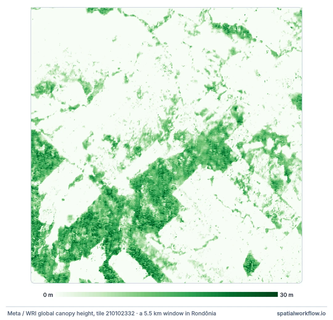
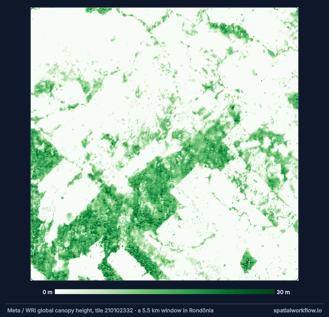
tile 210102332: 4660 × 4742 pixels of 1.19 m (Web Mercator)
canopy height percentiles 10/50/90/99: [ 0.  0. 15. 22.] m
share of pixels taller than  2 m: 34%
share of pixels taller than  5 m: 28%
share of pixels taller than 15 m: 8%
share of pixels taller than 25 m: 0%

Two-thirds of this window is under 2 m — pasture, cleared both before 2000 and since — and the rest splits into tall mature forest and lower regrowth, a mix that tree cover alone would call "forest" or "not forest".

Canopy height map of a 5.5 km window in Rondônia: most of it pale, under 2 metres, with dark green blocks of tall forest along a diagonal band and in the south-west, and lighter green patches of lower regrowth. — The window from the code above at about 5 m resolution. The pale ground is pasture; the dark diagonal band and the south-west corner are mature forest, mostly 15–22 m, and the paler greens in between are regrowth that a percent-cover map would call forest.

Find the tile, read in its CRS, mind Web Mercator pixels

1. Find the tile

The Meta/WRI map is split into zoom-9 Web Mercator tiles named by quadkey. Compute the quadkey for the centre of your area; areas near tile edges need two tiles.

2. Read a window in the tile's CRS

The tiles are EPSG:3857 at about 1.2 m. Transform your bounds into that CRS before computing the window. Tiles are organised in strips, so read short, wide windows where possible.

3. Mind the pixel size in Web Mercator

A Web Mercator "metre" is larger than a ground metre away from the equator by 1/cos(latitude). At 10°S the difference is 1.5%; at 50°N, 55%. Correct areas accordingly or reproject.

4. Aggregate to the resolution of your other data

To compare with 30 m products, resample by averaging (or taking the maximum, for canopy top height) onto their grid.

5. Treat heights as estimates

The model saturates in the tallest forests and smooths edges. Use heights for classes (regrowth vs mature, above 5 m or not) more than for exact values.

Tile, window, resolution, comparison.

Heights on the Hansen grid

The data used on this page

The Rondônia window used throughout the forest guides (63.0°–62.5°W, 10.8°–10.3°S): Hansen Global Forest Change v1.12 — tree cover in 2000, the year of loss, and the data mask — read from Google's storage into a three-band rondonia_gfc.tif, as in the Hansen reading guide.

import os

import rasterio
from rasterio.windows import from_bounds

W, S, E, N = -63.0, -10.8, -62.5, -10.3
V = "GFC-2024-v1.12"
if not os.path.exists("rondonia_gfc.tif"):
    bands = []
    for name in ("treecover2000", "lossyear", "datamask"):
        url = f"https://storage.googleapis.com/earthenginepartners-hansen/{V}/Hansen_{V}_{name}_10S_070W.tif"
        with rasterio.open(url) as src:
            window = from_bounds(W, S, E, N, src.transform)
            bands.append(src.read(1, window=window))
            profile = src.profile | {"count": 3, "width": bands[0].shape[1], "height": bands[0].shape[0],
                                     "transform": src.window_transform(window), "compress": "deflate",
                                     "driver": "GTiff", "tiled": False}
    profile.pop("blockxsize", None)
    profile.pop("blockysize", None)
    with rasterio.open("rondonia_gfc.tif", "w", **profile) as dst:
        for i, band in enumerate(bands, start=1):
            dst.write(band, i)
with rasterio.open("rondonia_gfc.tif") as src:
    print(src.count, src.shape, src.crs, src.res)

3 (2000, 2000) EPSG:4326 (0.00025, 0.00025)

Example 1 — heights on the Hansen grid

from rasterio.warp import reproject, Resampling
with rasterio.open("rondonia_gfc.tif") as src:
    gwin = from_bounds(W, S, E, N, src.transform)
    tc = src.read(1, window=gwin)
    ly = src.read(2, window=gwin)
    gtf = src.window_transform(gwin)
h30 = np.zeros(tc.shape, dtype="float32")
reproject(chm, h30, src_transform=chm_tf, src_crs=chm_crs, dst_transform=gtf,
          dst_crs="EPSG:4326", resampling=Resampling.average)
groups = {"forest 2000, never lost": (tc > 30) & (ly == 0),
          "forest 2000, lost 2001–10": (tc > 30) & (ly >= 1) & (ly <= 10),
          "forest 2000, lost 2011–24": (tc > 30) & (ly >= 11),
          "not forest in 2000": tc <= 30}
for name, m in groups.items():
    if m.sum():
        print(f"{name:<28} {m.mean():5.0%} of pixels, median height {np.median(h30[m]):5.1f} m, "
              f"share > 5 m {(h30[m] > 5).mean():5.0%}")

forest 2000, never lost        25% of pixels, median height   8.9 m, share > 5 m   59%
forest 2000, lost 2001–10      14% of pixels, median height   0.0 m, share > 5 m   14%
forest 2000, lost 2011–24      18% of pixels, median height   4.1 m, share > 5 m   46%
not forest in 2000             42% of pixels, median height   0.0 m, share > 5 m    6%

Forest never lost is the tallest group, and land cleared in 2001–10 is mostly bare — median 0 m, only 14% above 5 m. Land cleared in 2011–24 still has a median of 4 m and nearly half of it above 5 m, and that is a dating problem, not regrowth. The canopy height map is built from imagery taken over several years, largely before the most recent clearings, so forest cleared late in the record still stands in it. Before combining a height map with loss years, find out when its imagery was taken.

Example 2 — the 5 m criterion in a forest definition

f_cover = tc > 30
f_both = f_cover & (h30 > 5)
print(f"forest by canopy cover only (2000): {f_cover.mean():.0%} of the window")
print(f"cover > 30% in 2000 and height > 5 m in the recent canopy map: {f_both.mean():.0%}")
standing = (ly == 0) & f_cover
print(f"of the forest never lost, share under 5 m in the height map: {(h30[standing] <= 5).mean():.1%}")

forest by canopy cover only (2000): 58% of the window
cover > 30% in 2000 and height > 5 m in the recent canopy map: 26%
of the forest never lost, share under 5 m in the height map: 40.7%

Where the two disagree on land that was never recorded as lost, either the height model underestimates short but real forest, or the forest was degraded without a stand-replacing loss event. Both are worth a look on imagery.

Example 3 — regrowth on old clearings

old = (tc > 30) & (ly >= 1) & (ly <= 6)                         # cleared 2001–2006
print(f"cleared 2001–06: {old.mean():.0%} of the window")
for lo, hi in ((0, 2), (2, 5), (5, 10), (10, 60)):
    band = ((h30[old] > lo) | (lo == 0)) & (h30[old] <= hi)          # 0–2 m includes bare ground
    print(f"  now {lo:>2}–{hi:<2} m tall: {band.mean():.0%}")

cleared 2001–06: 13% of the window
  now  0–2  m tall: 77%
  now  2–5  m tall: 9%
  now  5–10 m tall: 9%
  now 10–60 m tall: 5%

Three-quarters of the 2001–06 clearings are under 2 m in the height map — still pasture — and one in seven has woody regrowth above 5 m. That regrowth is invisible in loss-only data and matters for carbon and connectivity.

Height tells mature forest, regrowth and pasture apart.

Height adds what cover misses

Why height adds what cover misses

Canopy cover saturates quickly: young regrowth closes its canopy in a few years and looks like forest in cover terms. Height keeps rising for decades. A height map therefore separates young from old forest, which matters for biomass, biodiversity and whether land meets a forest definition's height criterion.

Why the maps are model outputs

No satellite measures canopy height everywhere directly. GEDI lidar samples heights along tracks; airborne lidar covers small areas; imagery covers everything. The global maps train models on the lidar and apply them to imagery, so errors grow where training data were sparse and in structurally unusual forest.

Why the epoch matters

The Meta/WRI map represents imagery mostly from around 2018–2020; heights on land cleared later reflect the forest before clearing. Compare it with loss data only with that date in mind.

Regrowth that loss-only data never shows.

Tile sizes, no-data and tall forests

Tile size: each tile is 65,536 × 65,536 pixels; never read one whole.
No-data: water and missing imagery appear as 0 or no-data depending on the product; check before averaging.
ETH Global Canopy Height (10 m, 2020) is an alternative with uncertainty layers.
Area in Web Mercator: multiply pixel areas by cos²(latitude) for ground area, or reproject.
Tall forests: maps saturate around 30–40 m; do not read small differences among tall stands.

Internal links

How to build a canopy height model from lidar — the airborne alternative
Forest definitions explained — the 5 m criterion
How to read Hansen Global Forest Change data — cover and loss
Global Forest Change explained — why regrowth is missing there
Raster resampling explained — averaging to a coarser grid
Web Mercator distortion — why 3857 metres are not ground metres

FAQ

Where can I get global canopy height data?

The Meta/WRI 1 m map on AWS (dataforgood-fb-data), ETH Zurich's 10 m map, and GEDI-derived products.

How do I find the right tile?

Compute the zoom-9 quadkey of your location; the tile is chm/{quadkey}.tif.

Is the canopy height accurate?

It is a model estimate, good for distinguishing height classes, weaker in tall forests and at edges.

How do I compare it with 30 m data?

Reproject to the 30 m grid with average or maximum resampling.

Can canopy height show regrowth after clearing?

Yes — that is one of its main uses alongside loss data.

What year does the map represent?

Mostly imagery from around 2018–2020 for the Meta/WRI map; check the metadata for your tile.