
How to Read Hansen Global Forest Change Data in Python
On this page
Problem statement
The Hansen/UMD Global Forest Change dataset maps tree cover in 2000 and the year each 30 m pixel lost it since, for the whole land surface. It is the default starting point for any deforestation analysis, and it is distributed as 10° × 10° GeoTIFF tiles of 40,000 × 40,000 pixels — one file per layer per tile, several hundred megabytes each.
Nobody needs a whole tile. The practical workflow reads a window straight from Google Cloud Storage, keeps the four layers aligned, and converts pixel counts to areas that account for pixels shrinking towards the poles.
Quick answer
Open each layer through /vsicurl/, read the same window, and compute areas with a latitude-dependent pixel size:
import numpy as np, rasterio
from rasterio.windows import from_bounds

V = "GFC-2024-v1.12"
TILE = "10S_070W"                                # named by its top-left corner: 10°S, 70°W
W, S, E, N = -63.0, -10.8, -62.5, -10.3          # a 0.5° window in Rondônia, Brazil

def layer(name):
    url = (f"/vsicurl/https://storage.googleapis.com/earthenginepartners-hansen/"
           f"{V}/Hansen_{V}_{name}_{TILE}.tif")
    with rasterio.open(url) as src:
        win = from_bounds(W, S, E, N, src.transform)
        return src.read(1, window=win), src.window_transform(win)

treecover, tf = layer("treecover2000")           # % canopy closure in 2000, 0–100
lossyear, _ = layer("lossyear")                  # 0 = no loss, 1–24 = 2001–2024
datamask, _ = layer("datamask")                  # 1 = land, 2 = water, 0 = no data

lat = N - (np.arange(treecover.shape[0]) + 0.5) * abs(tf.e)
px_km2 = (abs(tf.a) * 111.320 * np.cos(np.radians(lat))) * (abs(tf.e) * 110.574)
area = np.broadcast_to(px_km2[:, None], treecover.shape)

forest = (treecover > 30) & (datamask == 1)
lost = forest & (lossyear > 0)
print(f"window: {treecover.shape[1]} × {treecover.shape[0]} pixels, {area.sum():,.0f} km²")
print(f"forest in 2000 (> 30% canopy): {area[forest].sum():,.0f} km²")
print(f"of which lost by 2024: {area[lost].sum():,.0f} km² ({area[lost].sum() / area[forest].sum():.0%})")
window: 2000 × 2000 pixels, 3,025 km²
forest in 2000 (> 30% canopy): 1,397 km²
of which lost by 2024: 613 km² (44%)
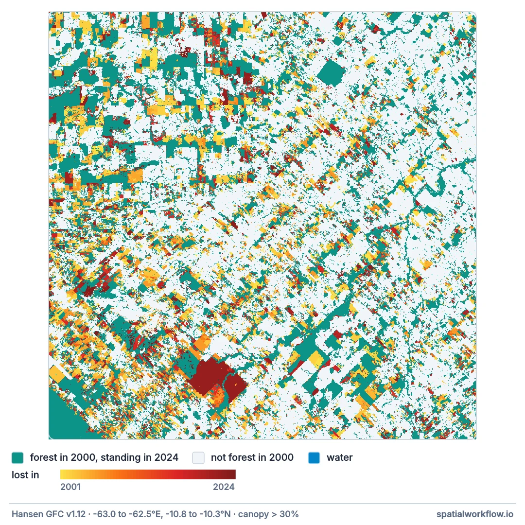
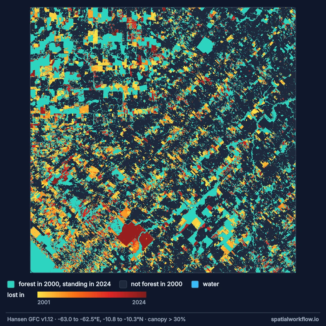
Four lines of setup and the headline numbers for a 3,000 km² window. Rondônia's "fishbone" deforestation along settlement roads shows up plainly: 44% of the forest standing in 2000 was lost by 2024.
Find the tile, read a window, threshold the cover
1. Find the tile
Tiles are named by their top-left corner: 10S_070W covers 10°S–20°S and 70°W–60°W. A study area that crosses a tile edge needs two reads and a mosaic.
2. Read a window, not the file
The tiles are stored in strips one row high, so a window read fetches whole rows across the tile — tens of megabytes for a 0.5° window rather than hundreds for the tile. from_bounds computes the window.
3. Read the layers you need, on the same window
treecover2000, lossyear, gain and datamask share the grid. Reading them with the same bounds keeps them pixel-aligned.
4. Define forest with a canopy threshold
Tree cover is a percentage. Forest is a threshold on it — commonly 10%, 25% or 30% — and the choice changes the forest area substantially. State it.
5. Convert pixels to area with latitude
The grid step is 0.00025°: at 10°S a pixel is about 27 × 28 m; at 60°N it is 14 × 28 m. Multiply each row's pixel count by that row's pixel area.
6. Mask water and no-data
datamask separates land from permanent water. Tree cover over water is zero, but loss statistics over a region should still use land area as the denominator.
Loss per year and an aligned stack
Example 1 — loss per year
years = np.arange(2001, 2025)
per_year = np.array([area[forest & (lossyear == y - 2000)].sum() for y in years])
for y, a in zip(years, per_year):
    if y in (2001, 2004, 2008, 2012, 2016, 2019, 2021, 2024):
        print(f"{y}: {a:6.1f} km²")
print(f"peak year {years[per_year.argmax()]} ({per_year.max():.0f} km²), "
      f"lowest {years[per_year.argmin()]} ({per_year.min():.0f} km²)")
2001: 77.6 km²
2004: 36.9 km²
2008: 14.0 km²
2012: 4.6 km²
2016: 19.8 km²
2019: 16.3 km²
2021: 17.4 km²
2024: 16.5 km²
peak year 2002 (97 km²), lowest 2012 (5 km²)
Loss peaked in 2002 at 97 km², fell twentyfold to 2012, and has run at 15–20 km² a year since 2016. The annual series is what most reporting uses. Its shape reflects policy, prices and enforcement — and, as the fix guide explains, changes in the algorithm between years.
Example 2 — the gain layer and what it can say
gain, _ = layer("gain")
print(f"gain pixels (2000–2012): {area[gain == 1].sum():.1f} km²")
print(f"gain on pixels that were also lost: {area[(gain == 1) & (lossyear > 0)].sum():.1f} km²")
gain pixels (2000–2012): 21.8 km²
gain on pixels that were also lost: 12.8 km²
More than half of the gain pixels — 12.8 of 21.8 km² — are also marked as lost: cleared and regrown, or regrown and cleared, on the same pixel. Gain covers only 2000–2012 and is a single flag, not a year. It cannot be subtracted from a 2001–2024 loss total to give "net" change.
Example 3 — save an aligned stack
profile = {"driver": "GTiff", "height": treecover.shape[0], "width": treecover.shape[1],
           "count": 3, "dtype": "uint8", "crs": "EPSG:4326", "transform": tf,
           "compress": "deflate", "tiled": True}
with rasterio.open("rondonia_gfc.tif", "w", **profile) as dst:
    for i, (arr, desc) in enumerate(((treecover, "treecover2000"), (lossyear, "lossyear"),
                                     (datamask, "datamask")), start=1):
        dst.write(arr, i)
        dst.set_band_description(i, desc)
print(f"saved {profile['width']} × {profile['height']} × 3 bands")
saved 2000 × 2000 × 3 bands
A local, tiled, compressed stack is a few megabytes and makes every later step fast. Keep the version (GFC-2024-v1.12) in the file name or metadata.
Cheap window reads and versions
Why a window read is cheap enough
GDAL's /vsicurl/ reads byte ranges over HTTP. With strip-organised tiles each window needs the full width of the rows it covers, so reading a narrow tall window is inefficient and a wide short one is not. For areas spanning many degrees, download the tiles; for sub-tile areas, windowed reads avoid the download entirely.
Why "forest" needs a threshold
The dataset maps tree canopy cover, not forest. Forest definitions — FAO's 10% canopy on at least 0.5 ha, national definitions at 20–30% — are thresholds on it. Savannas, plantations and agroforestry sit near those thresholds, so the choice moves forest area and loss rates.
Why the version matters
Each annual release reprocesses recent years and sometimes the whole record with improved methods. Numbers from GFC-2023 and GFC-2024 for the same area and year can differ. Pin the version and cite it.
Tile edges, encoding and latitude-dependent areas
- Tile edges: mosaic with
rasterio.mergewhen a study area crosses 10° lines. - Loss year encoding: values are years minus 2000; 0 means no loss detected.
- Loss is stand-replacement disturbance, including plantation harvest and fire — not only deforestation.
- Latitude-dependent areas: for large areas, reproject to an equal-area CRS instead of multiplying by row area.
- Newer layers (primary forest, drivers of loss) are separate datasets with their own grids.
Internal links
- Global Forest Change explained — what the layers mean and do not mean
- How to calculate forest loss by year for a region — per-polygon statistics
- Forest area wrong in degrees — the pixel-area fix guide
- Forest definitions explained — thresholds and their consequences
- How to read a raster window with rasterio — windowed reading
- How to merge and mosaic rasters with rasterio — areas across tile edges
FAQ
Where can I download Hansen forest change data?
From Google Cloud Storage (earthenginepartners-hansen) as 10° GeoTIFF tiles, or through Google Earth Engine.
How do I read only part of a tile?
Open it through /vsicurl/ with rasterio and read a window computed with from_bounds.
What does the lossyear value mean?
The year of stand-replacing loss minus 2000; 0 means no loss detected.
How do I calculate forest area correctly?
Multiply pixel counts by pixel area, which depends on latitude for a degree grid, or reproject to an equal-area CRS.
What tree cover threshold defines forest?
It depends on the definition you adopt: 10% (FAO), 25% or 30% are common. State it.
Can I compute net forest change from gain and loss?
No. Gain covers only 2000–2012 and is not dated; loss covers 2001 onward.