
How to Relate Land Surface Temperature to Vegetation in Python
On this page
Problem statement
Trees cool cities. That is the conclusion of hundreds of studies, and most of them show it the same way: a scatter plot of surface temperature against NDVI with a downward slope. The relationship is real, and the slope is easy to misread. NDVI and surface temperature are both computed from the same scenes, both depend on what else is in the pixel, and in a dry city the least vegetated surfaces are not always the hottest — bare soil in summer can outdo asphalt, and water has almost no NDVI and the lowest temperature of all.
A useful analysis separates land cover types before fitting anything, uses NDVI and LST from the same observations, and reports the slope with the classes it applies to.
Quick answer
Compute NDVI and LST on the same grid from the same scenes, then look at the relationship within land cover classes:
import numpy as np, rasterio, pystac_client, planetary_computer
from rasterio.warp import reproject, Resampling, transform_bounds
from rasterio.transform import from_origin

AOI = (-3.80, 40.35, -3.60, 40.50)                              # central Madrid
CRS = "EPSG:32630"
x0, y0, x1, y1 = transform_bounds("EPSG:4326", CRS, *AOI)
x0, y1 = np.floor(x0 / 30) * 30, np.ceil(y1 / 30) * 30
W, H = int(np.ceil((x1 - x0) / 30)), int(np.ceil((y1 - y0) / 30))
TF = from_origin(x0, y1, 30, 30)

cat = pystac_client.Client.open("https://planetarycomputer.microsoft.com/api/stac/v1")
items = [i for i in cat.search(collections=["landsat-c2-l2"], bbox=list(AOI),
                               datetime="2023-06-01/2023-08-31").items()
         if i.properties["platform"] in ("landsat-8", "landsat-9") and i.properties["eo:cloud_cover"] < 20]

def grid(item, asset):
    out = np.zeros((H, W), dtype="uint16")
    with rasterio.open(planetary_computer.sign(item.assets[asset].href)) as src:
        reproject(rasterio.band(src, 1), out, dst_transform=TF, dst_crs=CRS,
                  resampling=Resampling.nearest)
    return out.astype("float32")

lst_l, ndvi_l = [], []
for it in items:
    qa = grid(it, "qa_pixel").astype("uint16")
    bad = (((qa >> 1) & 1) | ((qa >> 3) & 1) | ((qa >> 4) & 1)).astype(bool) | (qa == 0)
    st = grid(it, "lwir11") * 0.00341802 + 149.0 - 273.15
    red = grid(it, "red") * 0.0000275 - 0.2                     # Collection 2 reflectance scale
    nir = grid(it, "nir08") * 0.0000275 - 0.2
    nd = (nir - red) / (nir + red)
    st[bad], nd[bad] = np.nan, np.nan
    lst_l.append(st); ndvi_l.append(nd)
lst = np.nanmedian(np.stack(lst_l), axis=0)
ndvi = np.nanmedian(np.stack(ndvi_l), axis=0)
ok = np.isfinite(lst) & np.isfinite(ndvi)
slope, intercept = np.polyfit(ndvi[ok], lst[ok], 1)
print(f"{len(items)} scenes; {ok.sum():,} pixels")
print(f"all pixels: LST = {intercept:.1f} {slope:+.1f} × NDVI  (r = {np.corrcoef(ndvi[ok], lst[ok])[0, 1]:.2f})")
8 scenes; 319,549 pixels
all pixels: LST = 46.8 -8.4 × NDVI (r = -0.37)
A clear but moderate negative relationship across the whole city: 8.4 °C cooler per unit of NDVI, about 0.8 °C per 0.1, with r = −0.37. The correlation is modest because many other things set surface temperature too. The next step is finding out where along the NDVI range that slope actually comes from.
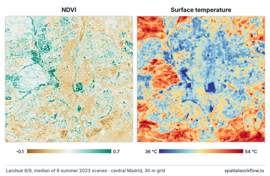
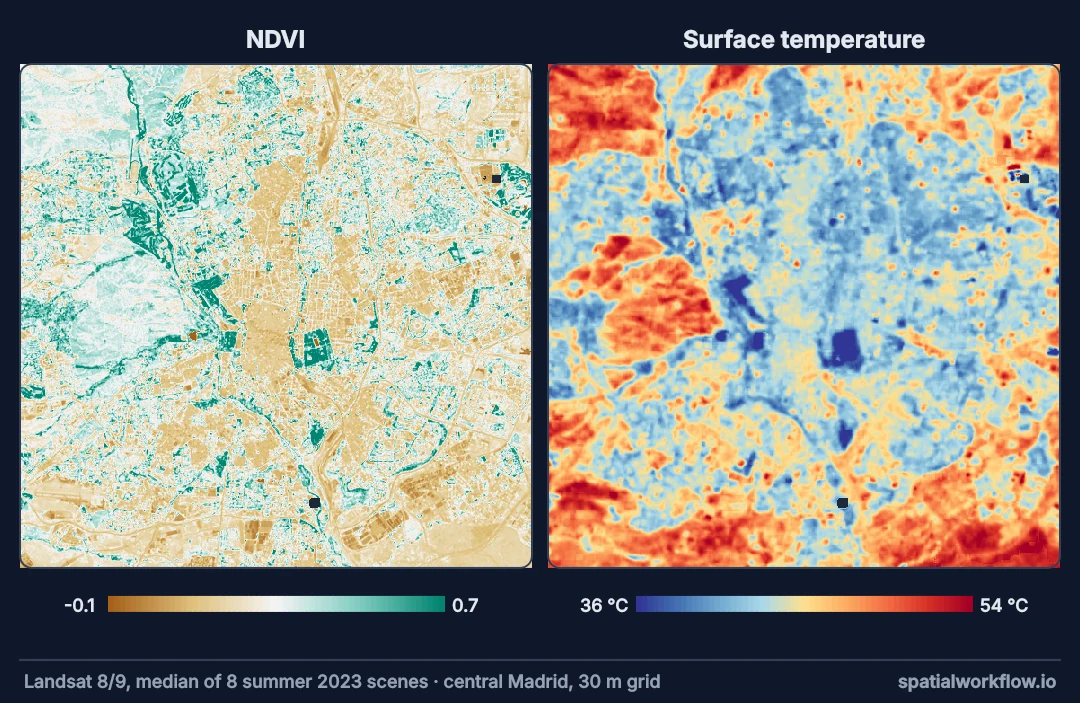
Same scenes, right scales, split by cover, bin
1. Use the same scenes for both variables
NDVI from a spring image and LST from a summer one relate two different states of the city. Compute both from the same observations, then composite.
2. Apply the right scale factors
Collection 2 surface reflectance is DN × 0.0000275 − 0.2; surface temperature is DN × 0.00341802 + 149.0 K. Different bands, different factors.
3. Split by land cover
Water, bare soil, built-up, grassland and trees behave differently. Fit or summarise within classes before drawing a single line through all of them.
4. Bin rather than scatter
With hundreds of thousands of pixels, a binned mean (LST by NDVI decile) shows the shape of the relationship more clearly than a cloud of points, including any non-linearity.
5. Report the slope per unit that means something
"−15 °C per unit NDVI" is abstract; "a 0.1 increase in NDVI goes with 1.5 °C cooler surfaces" is readable.
Cooling per step of NDVI in built-up areas
Example 1 — LST by NDVI bin
bins = np.arange(-0.1, 0.85, 0.1)
idx = np.digitize(ndvi[ok], bins)
for i in range(1, len(bins)):
    m = idx == i
    if m.sum() > 500:
        print(f"NDVI {bins[i - 1]:+.1f}–{bins[i]:+.1f}: {m.sum():>7,} px, median LST {np.median(lst[ok][m]):5.1f} °C")
NDVI -0.1–+0.0: 961 px, median LST 47.0 °C
NDVI +0.0–+0.1: 21,707 px, median LST 44.8 °C
NDVI +0.1–+0.2: 84,204 px, median LST 44.6 °C
NDVI +0.2–+0.3: 86,360 px, median LST 44.5 °C
NDVI +0.3–+0.4: 67,340 px, median LST 44.0 °C
NDVI +0.4–+0.5: 32,591 px, median LST 42.4 °C
NDVI +0.5–+0.6: 14,214 px, median LST 41.3 °C
NDVI +0.6–+0.7: 7,535 px, median LST 40.3 °C
NDVI +0.7–+0.8: 3,899 px, median LST 39.1 °C
The binned curve is not a straight line. From NDVI 0 to 0.4 — most of the city fabric — surface temperature barely moves, from 44.8 to 44.0 °C. Above 0.4 it falls steeply, to 39.1 °C in the greenest pixels: parks and dense tree canopy. The cooling is concentrated where vegetation dominates the pixel, not spread evenly across the range.
Example 2 — within land cover classes
wc = np.zeros((H, W), dtype="uint8")
for it in cat.search(collections=["esa-worldcover"], bbox=list(AOI), datetime="2021").items():
    with rasterio.open(planetary_computer.sign(it.assets["map"].href)) as src:
        tmp = np.zeros((H, W), dtype="uint8")
        reproject(rasterio.band(src, 1), tmp, dst_transform=TF, dst_crs=CRS, resampling=Resampling.mode)
        wc = np.where(wc == 0, tmp, wc)
for code, name in ((10, "tree cover"), (30, "grassland"), (50, "built-up"), (60, "bare"), (80, "water")):
    m = ok & (wc == code)
    if m.sum() > 300:
        s_, _ = np.polyfit(ndvi[m], lst[m], 1)
        print(f"{name:<11} {m.sum():>7,} px, median LST {np.median(lst[m]):5.1f} °C, "
              f"median NDVI {np.median(ndvi[m]):.2f}, slope {s_:+.1f} °C per NDVI unit")
tree cover 64,878 px, median LST 42.5 °C, median NDVI 0.41, slope -11.7 °C per NDVI unit
grassland 59,819 px, median LST 48.3 °C, median NDVI 0.27, slope -15.0 °C per NDVI unit
built-up 182,345 px, median LST 43.5 °C, median NDVI 0.21, slope -7.7 °C per NDVI unit
bare 3,273 px, median LST 45.4 °C, median NDVI 0.16, slope -8.4 °C per NDVI unit
water 565 px, median LST 38.0 °C, median NDVI 0.15, slope +7.0 °C per NDVI unit
Within classes the slopes differ: steeper than the citywide slope in grassland (−15.0 °C per NDVI unit) and tree cover (−11.7), shallower in built-up land (−7.7). Grassland is also the hottest class, at 48.3 °C: dry grass has a low NDVI and no water to spend, and the greener, watered patches are much cooler. Water runs the other way. The citywide slope blends all of these.
Example 3 — the cooling per 0.1 NDVI in built-up areas
m = ok & (wc == 50)
s_b, _ = np.polyfit(ndvi[m], lst[m], 1)
print(f"built-up pixels: each +0.1 NDVI goes with {s_b * 0.1:+.1f} °C surface temperature")
p10, p90 = np.percentile(ndvi[m], [10, 90])
print(f"built-up NDVI ranges {p10:.2f}–{p90:.2f} (10th–90th percentile): "
      f"a modelled difference of {s_b * (p90 - p10):+.1f} °C")
built-up pixels: each +0.1 NDVI goes with -0.8 °C surface temperature
built-up NDVI ranges 0.09–0.39 (10th–90th percentile): a modelled difference of -2.3 °C
Within built-up land, 0.1 more NDVI goes with 0.8 °C cooler surfaces, and the greenest built-up tenth is modelled 2.3 °C cooler than the least green. That within-class difference — the effect of more street trees and gardens among the same kind of buildings — is the number most relevant to greening policy.
Why vegetation cools, and citywide slopes overstate it
Why vegetation cools surfaces
Plants move water from the soil into the air through their leaves, and evaporation uses energy that would otherwise heat the surface. Trees add shade, cooling the ground beneath them too. A well-watered canopy stays close to air temperature while asphalt beside it runs 20 °C hotter.
Why a citywide slope overstates the effect of greening
Across a whole city, NDVI separates surface types — water, roofs, parks — whose temperatures differ for many reasons besides vegetation. Planting trees in a street changes NDVI within the built-up class, where the relationship is weaker. The within-class slope is the relevant one for interventions.
Why the Mediterranean summer matters
In a dry summer, unirrigated grass browns and its NDVI falls; its surface then heats nearly as much as bare soil. Irrigated parks stay green and cool. The same vegetation index means different cooling in different seasons and water regimes.
Water, shadows and causality
- Water has negative NDVI and low LST; exclude it or treat it as a class, or it dominates the fit.
- Shadows from tall buildings lower both reflectance and LST; they look like cool vegetation in some indices.
- Resolution: LST is 100 m native; NDVI is 30 m. Aggregate NDVI to 90–100 m for a fair pixel-level comparison.
- Causality: correlation across pixels is not the effect of planting; affluent neighbourhoods have both more trees and other differences.
- Other indices: fractional vegetation cover or impervious surface fraction often explain LST better than NDVI.
Internal links
- Urban cooling and green space explained — the physics and the evidence
- How to measure the cooling effect of parks — distance from parks
- How to calculate NDVI in Python — the index
- How to read Landsat surface temperature — the LST input
- LST resolution misread — why 30 m LST is really 100 m
- How to calculate surface urban heat island intensity — the city-scale view
FAQ
Does vegetation lower land surface temperature?
Yes — through evaporation and shade. The size of the effect depends on the vegetation type, its water supply and what it replaces.
How do I compute NDVI and LST from the same Landsat scene?
Scale red and NIR by 0.0000275 and −0.2 for reflectance; scale the thermal band by 0.00341802 and +149 for Kelvin; mask with QA_PIXEL.
Why isn't the LST–NDVI relationship linear?
Water, bare soil and roofs sit at the low-NDVI end with very different temperatures.
Should I fit one regression for the whole city?
Fit within land cover classes; the citywide slope mixes surface types.
What slope is typical?
Here about 0.8 °C per 0.1 NDVI, both citywide and within built-up land, and much more in the greenest pixels — measure it for your city and season.
Does correlation show that planting trees will cool a street?
Not by itself; within-class comparisons and before-and-after studies are closer to that question.