
How to build a landslide susceptibility index in Python
On this page
Problem statement
Building a susceptibility layer is a weighted overlay: derive factors from a DEM and a land-cover map, rescale each to a common range, weight them, and classify the sum. Every step has a decision in it — where each factor saturates, how the weights are set, whether the classes are quantiles or fixed breaks — and the resulting map looks equally authoritative whichever choices were made.
This guide builds a post-fire debris-flow susceptibility index for ground inside the 2024 Park Fire: slope and curvature from the Copernicus DEM, burn severity from Sentinel-2, and land cover from WorldCover. It also shows what the map cannot say without an inventory of past failures, and what changes when the weights change.
Quick answer
Derive the factors, rescale, weight, and keep every intermediate layer:
import numpy as np, pystac_client, planetary_computer, rasterio
from rasterio.enums import Resampling
from rasterio.transform import from_origin
from rasterio.vrt import WarpedVRT
from rasterio.warp import transform_bounds

BBOX = [-122.00, 40.00, -121.74, 40.22]
CRS, RES = "EPSG:32610", 20
left, bottom, right, top = transform_bounds(4326, CRS, *BBOX)
GRID = {"crs": CRS, "transform": from_origin(left, top, RES, RES),
        "width": int((right - left) // RES), "height": int((top - bottom) // RES)}
cat = pystac_client.Client.open("https://planetarycomputer.microsoft.com/api/stac/v1",
                                modifier=planetary_computer.sign_inplace)

def on_grid(item, asset, resampling=Resampling.bilinear):
    with rasterio.open(item.assets[asset].href) as src, WarpedVRT(
            src, crs=GRID["crs"], transform=GRID["transform"], width=GRID["width"],
            height=GRID["height"], resampling=resampling, nodata=np.nan) as vrt:
        return vrt.read(1)

dem = np.full((GRID["height"], GRID["width"]), np.nan, "float32")
for it in cat.search(collections=["cop-dem-glo-30"], bbox=BBOX).items():
    a = on_grid(it, "data")
    dem[np.isnan(dem) & np.isfinite(a)] = a[np.isnan(dem) & np.isfinite(a)]

gy, gx = np.gradient(dem, RES)
slope = np.degrees(np.arctan(np.hypot(gx, gy)))
curvature = np.gradient(np.gradient(dem, RES, axis=0), RES, axis=0) + \
            np.gradient(np.gradient(dem, RES, axis=1), RES, axis=1)
dnbr = np.load("dnbr.npy")                                   # severity, same grid

def rescale(x, lo, hi):
    return np.clip((x - lo) / (hi - lo), 0, 1)

factors = {"slope": rescale(slope, 10, 45),
           "severity": rescale(dnbr, 100, 650),
           "convergence": rescale(-curvature, 0, 0.05)}     # hollows collect water
weights = {"slope": 0.5, "severity": 0.3, "convergence": 0.2}
index = sum(weights[k] * factors[k] for k in factors)
print({k: round(float(np.nanmedian(v)), 3) for k, v in factors.items()})
print(f"index: median {np.nanmedian(index):.3f}, 95th percentile {np.nanpercentile(index, 95):.3f}")
{'slope': 0.121, 'severity': 0.179, 'convergence': 0.007}
index: median 0.139, 95th percentile 0.376
Each factor is on 0–1 after rescaling, so the weights are the only thing setting their relative influence — which is why they have to be stated.
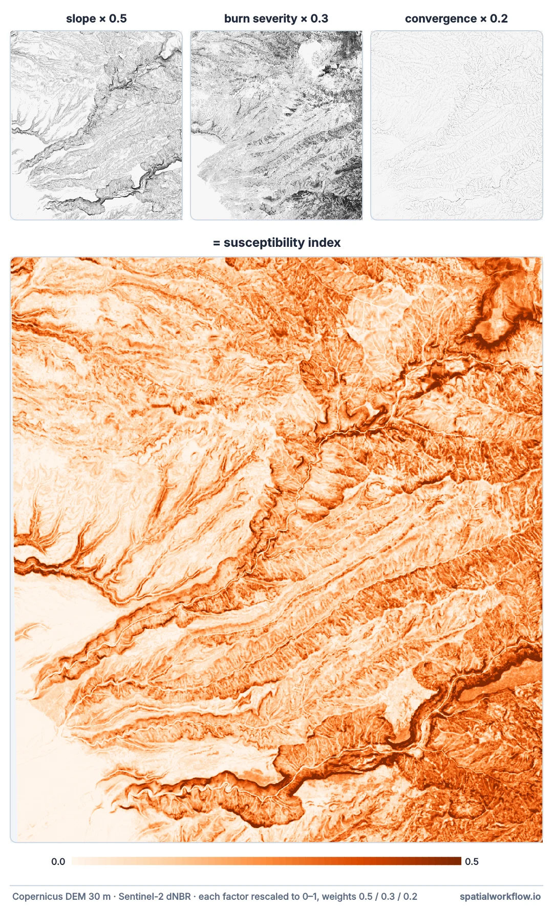
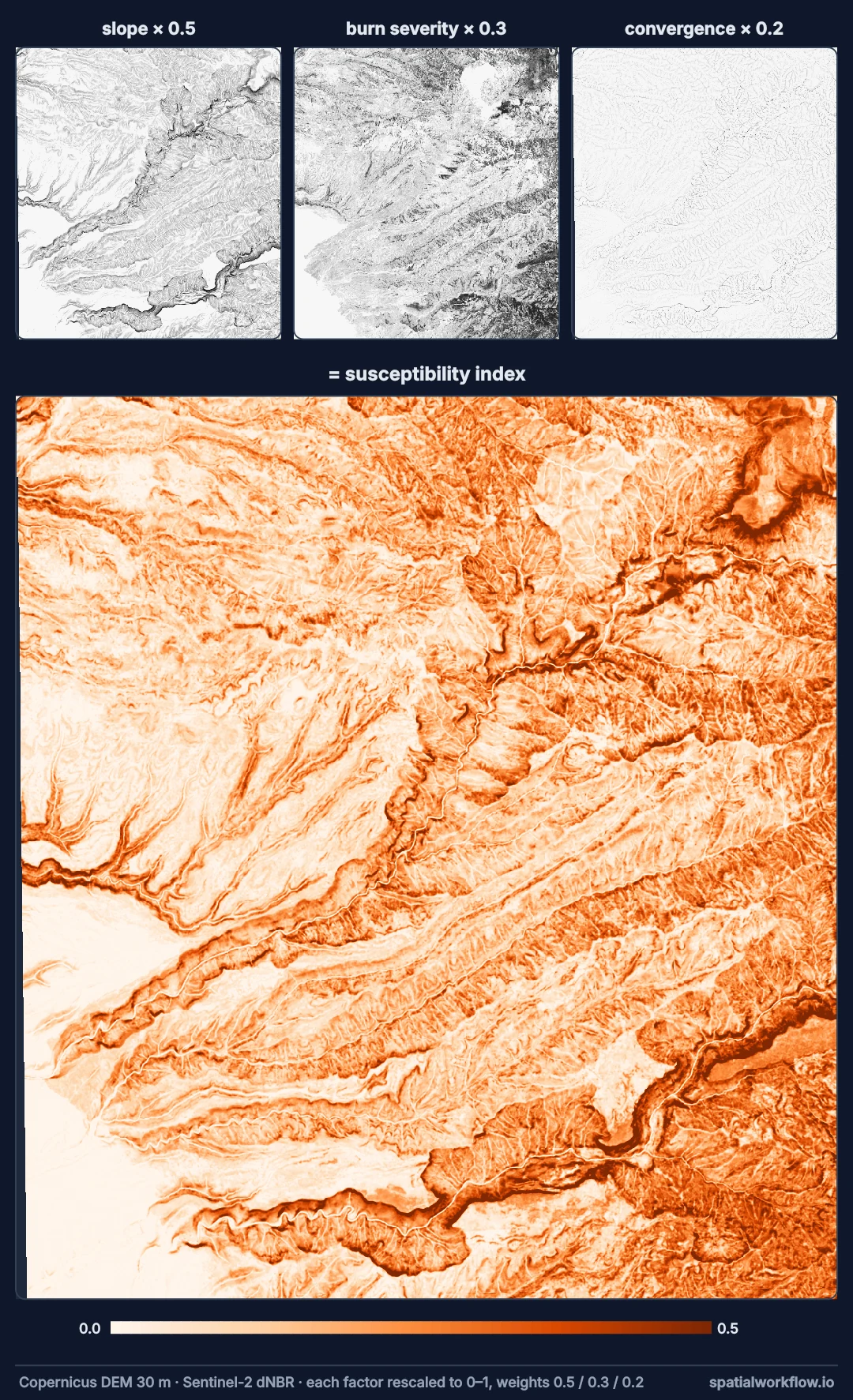
One grid, terrain factors, saturation points, weights
1. Put every factor on one grid
Same CRS, same resolution, same extent, so the arrays can be combined element-wise.
2. Derive terrain factors at a sensible resolution
Slope from a 30 m DEM is smoother than slope from a 2 m DEM, and debris flows start in small steep hollows. Say which DEM the factors came from.
3. Rescale with explicit saturation points
rescale(slope, 10, 45) says that below 10° slope contributes nothing and above 45° it contributes fully. Those two numbers are as important as the weight.
4. Weight, and test the weighting
Change the weights and see how much the top class moves. If it barely moves, the weights are not doing much; if it moves a lot, the map is an expression of them.
5. Classify by quantile or by fixed break — and say which
Quantile classes always fill the same share of the map. Fixed breaks let a genuinely low-susceptibility area come out mostly low.
6. Validate if you can, and label it if you cannot
With an inventory, report AUC on held-out ground. Without one, the honest label is "index", not "probability".
What each factor and weight contributes
The data used on this page
The 2024 Park Fire perimeter from the WFIGS interagency fire perimeters service (park_perimeter.geojson). The burn severity comes from How to map burn severity with dNBR: its two Sentinel-2 scenes (2 July and 10 September 2024) on the same 20 m window as the DEM here, saved as the uncorrected dNBR (dnbr.npy).
import os

import geopandas as gpd
import numpy as np
import pystac_client
import rasterio
import requests
from rasterio.enums import Resampling
from rasterio.transform import from_origin
from rasterio.vrt import WarpedVRT
from rasterio.warp import transform_bounds
from shapely.geometry import box, shape

WFIGS = ("https://services3.arcgis.com/T4QMspbfLg3qTGWY/arcgis/rest/services/"
         "WFIGS_Interagency_Perimeters/FeatureServer/0/query")
if not os.path.exists("park_perimeter.geojson"):
    reply = requests.get(WFIGS, params={"where": "poly_IncidentName='PARK' AND attr_POOState='US-CA'",
                                        "outFields": "*", "f": "geojson", "outSR": 4326}, timeout=300)
    reply.raise_for_status()
    open("park_perimeter.geojson", "w").write(reply.text)

if not os.path.exists("dnbr.npy"):
    BBOX = [-122.00, 40.00, -121.74, 40.22]
    left, bottom, right, top = transform_bounds(4326, "EPSG:32610", *BBOX)
    GRID = {"crs": "EPSG:32610", "transform": from_origin(left, top, 20, 20),
            "width": int((right - left) // 20), "height": int((top - bottom) // 20)}
    es = pystac_client.Client.open("https://earth-search.aws.element84.com/v1")

    def scene(dates):
        items = [i for i in es.search(collections=["sentinel-2-c1-l2a"], bbox=BBOX, datetime=dates,
                                      query={"eo:cloud_cover": {"lt": 5}}).item_collection()
                 if shape(i.geometry).contains(box(*BBOX))]
        return sorted(items, key=lambda i: i.datetime)[0]

    def band(item, name):
        with rasterio.open(item.assets[name].href) as src, WarpedVRT(
                src, crs=GRID["crs"], transform=GRID["transform"], width=GRID["width"],
                height=GRID["height"], resampling=Resampling.bilinear) as vrt:
            a = vrt.read(1).astype("float32")
        return np.where(a > 0, a * 0.0001, np.nan)

    def nbr(item):
        return (band(item, "nir08") - band(item, "swir22")) / (band(item, "nir08") + band(item, "swir22"))

    pre, post = scene("2024-07-01/2024-07-10"), scene("2024-09-08/2024-09-15")
    np.save("pre_nbr.npy", nbr(pre))
    np.save("dnbr.npy", (nbr(pre) - nbr(post)) * 1000)
print(np.load("dnbr.npy").shape, "dNBR grid")
(1235, 1123) dNBR grid
Example 1 — what each factor contributes
top = index >= np.nanpercentile(index, 95)
for name, f in factors.items():
    print(f"{name:12} median in top 5%: {np.nanmedian(f[top]):.2f}   "
          f"elsewhere: {np.nanmedian(f[~top]):.2f}")
print(f"top class: median slope {np.nanmedian(slope[top]):.1f}°, "
      f"median dNBR {np.nanmedian(dnbr[top]):.0f}")

# convergence contributes nothing: its saturation point was set far too high.
print("curvature percentiles:", np.round(np.nanpercentile(-curvature, [50, 90, 99]), 4).tolist())
factors["convergence"] = rescale(-curvature, 0, float(np.nanpercentile(-curvature, 99)))
index = sum(weights[k] * factors[k] for k in factors)
top = index >= np.nanpercentile(index, 95)
print(f"rescaled: convergence median in top 5% {np.nanmedian(factors['convergence'][top]):.2f}, "
      f"elsewhere {np.nanmedian(factors['convergence'][~top]):.2f}")
slope median in top 5%: 0.51 elsewhere: 0.11
severity median in top 5%: 0.62 elsewhere: 0.17
convergence median in top 5%: 0.01 elsewhere: 0.01
top class: median slope 27.8°, median dNBR 439
curvature percentiles: [0.0003, 0.0056, 0.0132]
rescaled: convergence median in top 5% 0.30, elsewhere 0.02
A factor that has the same median inside and outside the top class is not doing anything. Here the first attempt saturated convergence at a curvature of 0.05, against a 99th percentile of 0.013 and a median of 0.0003, so almost every pixel scored near zero on it and the weight of 0.2 bought nothing. Rescaling to the data's own 99th percentile brings the factor back into play: its median is then 0.30 in the top class against 0.02 elsewhere.
Example 2 — how much the weights matter
schemes = {"slope-led": {"slope": 0.5, "severity": 0.3, "convergence": 0.2},
           "severity-led": {"slope": 0.3, "severity": 0.5, "convergence": 0.2},
           "equal": {"slope": 1 / 3, "severity": 1 / 3, "convergence": 1 / 3}}
tops = {}
for name, w in schemes.items():
    idx = sum(w[k] * factors[k] for k in factors)
    tops[name] = idx >= np.nanpercentile(idx, 95)
    print(f"{name:13} top 5% covers {np.nansum(tops[name]) * RES * RES / 1e6:5.1f} km²")
base = tops["slope-led"]
for name, t in tops.items():
    overlap = np.nansum(t & base) / np.nansum(base)
    print(f"  agreement with slope-led: {name:13} {overlap:5.1%}")
slope-led top 5% covers 27.5 km²
severity-led top 5% covers 27.5 km²
equal top 5% covers 27.5 km²
agreement with slope-led: slope-led 100.0%
agreement with slope-led: severity-led 61.1%
agreement with slope-led: equal 71.2%
Example 3 — write it out with its parameters
profile = dict(driver="GTiff", dtype="float32", count=1, crs=GRID["crs"],
               transform=GRID["transform"], width=GRID["width"], height=GRID["height"],
               nodata=np.nan, compress="deflate", tiled=True)
with rasterio.open("park_debris_flow_index.tif", "w", **profile) as dst:
    dst.write(index.astype("float32"), 1)
    dst.update_tags(product="susceptibility index (not probability)",
                    factors="slope 10-45deg; dNBR 100-650; convergence 0-0.05",
                    weights="slope 0.5; severity 0.3; convergence 0.2",
                    dem="Copernicus DEM GLO-30", severity="Sentinel-2 dNBR 2024-07-02/2024-09-10",
                    validation="none: no landslide inventory available")
import os
print(f"{os.path.getsize('park_debris_flow_index.tif') / 1e6:.1f} MB written")
with rasterio.open("park_debris_flow_index.tif") as src:
    print({k: v for k, v in src.tags().items() if k in ("product", "validation")})
4.8 MB written
{'product': 'susceptibility index (not probability)', 'validation': 'none: no landslide inventory available'}
Rescaling points matter as much as weights
Why the rescaling points matter as much as the weights
A factor rescaled to saturate at 45° contributes its full weight on every slope steeper than that, so in terrain where most slopes exceed 45° it becomes a constant and stops discriminating. The saturation points set where in the landscape a factor still varies, which is where it can still influence the ranking.
Why weight sensitivity is the cheapest validation available
With no inventory there is nothing to test against, but there is still something to measure: how much the map depends on the arbitrary parts. Recomputing the top class under different weightings and reporting the overlap tells a reader how much of the map is data and how much is opinion.
Why post-fire is a special case
Burned catchments produce debris flows at rainfall intensities that would do nothing before the fire, and the elevated risk fades over a few years as vegetation returns. That makes burn severity a genuine factor with a physical mechanism — and it makes the map's validity time-limited in a way a geological susceptibility map is not.
Source versus runout, rainfall and cut slopes
- Source and runout are different questions; this index maps where flows start.
- Rainfall thresholds turn susceptibility into a warning system; USGS publishes them for burned areas.
- Curvature is noisy on a 30 m DEM; smooth it before rescaling if the map looks speckled.
- Roads and cut slopes are strong factors where the data exists.
- Time limit: post-fire susceptibility decays; date the map and say for how long it applies.
- Do not classify into "risk"; there is no exposure or vulnerability in this layer.
Internal links
- Landslide susceptibility explained — what the map is and is not
- Burn severity explained — the severity factor
- How to map burn severity with dNBR in Python — producing it
- Site suitability explained — the same weighted-overlay machinery
- How to run a weighted site suitability analysis in Python — weights and rescaling in detail
- How to calculate slope and aspect in Python — the terrain factors
FAQ
How do I build a landslide susceptibility map in Python?
Derive factors onto one grid, rescale each to 0–1 with explicit saturation points, weight them, and classify — recording every parameter.
Where do the weights come from?
Expert judgement, or fitted to an inventory. Without an inventory, test how much the map depends on them.
Should I use quantile or fixed classes?
Fixed breaks if you want low-susceptibility areas to be able to come out low; quantiles if you want a fixed share in each class. Say which.
Is burn severity a real factor?
For debris flows after fire, yes — burned ground generates runoff at much lower rainfall intensities.
Can I call the output a probability?
No. Without an inventory and a frequency, it is a ranking.
How long does a post-fire map stay valid?
A few years at most; vegetation recovery reduces the effect.