Flood hazard maps explained: depth, extent and which flood they describe

Problem statement

A flood hazard map is usually read as "the area that floods". It is not. It is the area that a particular model, driven by a particular scenario, says would be under water — with a depth at every point, for one return period, from one flood source, under the land surface and defences as they were when the model ran. Change any of those and the blue area moves.

The Valencia flood of October 2024 makes the point. The European Commission's continental flood hazard map puts 78.7 km² — 24% of a window south of the city — under water in a 1-in-100-year fluvial flood, with depths up to 13.6 m. Sentinel-1 mapped 31.6 km² of new open water three days after the real event. Just under half of that observed water lies inside the modelled zone, and three quarters of the modelled zone was not wet. Neither map is wrong: they answer different questions.

Quick answer

Read the depth grid, not just the outline, and keep the scenario attached to it:

import numpy as np, rasterio
from rasterio.windows import from_bounds
from rasterio.warp import transform_bounds

bbox = [-0.46, 39.25, -0.33, 39.45]                     # south of Valencia
path = "flood/floodmap_EFAS_RP100_C.tif"                # JRC EFAS, 100 m, depth in metres
with rasterio.open(path) as src:
    win = from_bounds(*transform_bounds(4326, src.crs, *bbox), src.transform)
    depth = src.read(1, window=win, masked=True).filled(np.nan)
    print("CRS", src.crs.to_epsg(), "| pixel", src.res[0], "m | nodata", src.nodata)

flooded = depth > 0
print(f"flooded area {flooded.sum() * 0.01:.1f} km² ({flooded.mean():.1%} of the window)")
print("depth percentiles (m):", np.round(np.nanpercentile(depth[flooded], [50, 90, 99]), 2).tolist())

CRS None | pixel 100.0 m | nodata -3.4028230607370965e+38
flooded area 78.7 km² (24.1% of the window)
depth percentiles (m): [0.82, 2.01, 4.56]

to_epsg() returning None is worth noting: the file carries an ESRI-style WKT for ETRS89-LAEA rather than an EPSG code, which is why every read here reprojects the bounding box through the file's own CRS object rather than assuming a code.

Depth is what the map is for. An extent polygon alone cannot tell a 10 cm nuisance flood from two metres in a living room, and the damage functions that turn hazard into loss take depth as their input.

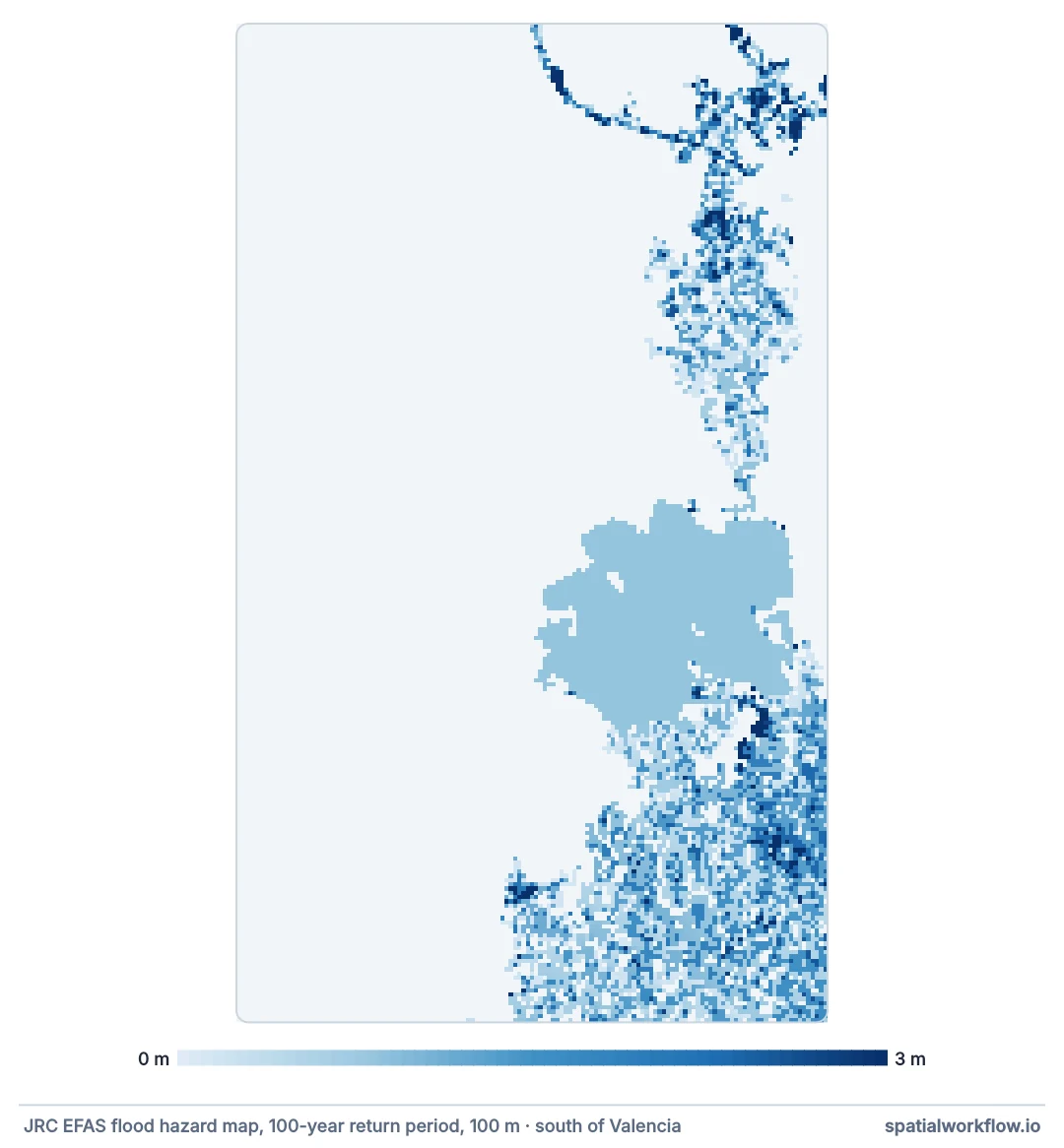
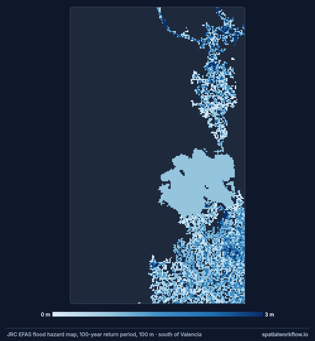
Which flood, which return period, defences, depth

1. Find out which flood the map is of

Fluvial (river), pluvial (rainfall on the spot), coastal (surge), or groundwater. Most continental maps are fluvial only, so they show nothing in a town flooded by its own drains.

2. Find the return period

A 1-in-10 map and a 1-in-500 map are both correct and look completely different. Return periods sets out what the number means.

3. Check whether defences are included

"Undefended" maps show the flood a river would cause with no levees or walls. Defended maps include them, and therefore need to be redrawn whenever a defence is built or fails.

4. Keep the depth, not just the outline

Depth drives damage. Keep the grid; derive the outline from it when a map needs one.

5. Check the terrain model and resolution

A 100 m continental map cannot see a 20 m-wide flood defence or a raised road. Local maps at 2–5 m from lidar can, which is why they disagree with continental ones in detail.

6. Do not read a hazard map as a forecast

It describes a scenario with an annual probability, not the next flood. The next flood will differ in source, duration and shape.

Modelled floods against an observed one

The data used on this page

The European Flood Awareness System's pan-European flood hazard maps from the JRC (data catalogue): water depth in metres on a 100 m grid for the 1-in-10, 1-in-100, 1-in-500-year floods, one zipped GeoTIFF per return period, saved under flood/.

import os
import zipfile

import requests

EFAS = "https://jeodpp.jrc.ec.europa.eu/ftp/jrc-opendata/FLOODS/EuropeanMaps/floodMap_RP{}.zip"
os.makedirs("flood", exist_ok=True)
for rp in ("010", "100", "500"):
    tif = f"floodmap_EFAS_RP{rp}_C.tif"
    if not os.path.exists(f"flood/{tif}"):                      # about 180 MB per return period
        with requests.get(EFAS.format(rp), stream=True, timeout=600) as r:
            r.raise_for_status()
            with open("efas.zip", "wb") as f:
                for chunk in r.iter_content(1 << 20):
                    f.write(chunk)
        zipfile.ZipFile("efas.zip").extract(tif, "flood")
        os.remove("efas.zip")
print(sorted(os.listdir("flood")))

['floodmap_EFAS_RP010_C.tif', 'floodmap_EFAS_RP100_C.tif', 'floodmap_EFAS_RP500_C.tif']

sar_io.py, the helper module from the reading guide.

%%writefile sar_io.py
"""Find, read and mosaic Sentinel-1 RTC scenes from Microsoft Planetary Computer."""
from collections import defaultdict

import numpy as np
import planetary_computer
import pystac_client
import rasterio
from rasterio.enums import Resampling
from rasterio.transform import from_origin
from rasterio.vrt import WarpedVRT
from rasterio.warp import transform_bounds

STAC = "https://planetarycomputer.microsoft.com/api/stac/v1"


def search(bbox, dates, orbit=None, direction=None, collection="sentinel-1-rtc"):
    """Items over bbox (lon/lat) in a date range, filtered by relative orbit and pass direction."""
    cat = pystac_client.Client.open(STAC, modifier=planetary_computer.sign_inplace)
    items = cat.search(collections=[collection], bbox=bbox, datetime=dates).item_collection()
    keep = [i for i in items
            if (orbit is None or i.properties["sat:relative_orbit"] == orbit)
            and (direction is None or i.properties["sat:orbit_state"] == direction)]
    return sorted(keep, key=lambda i: i.datetime)


def passes(items):
    """Group frames into passes: same day, same relative orbit."""
    groups = defaultdict(list)
    for i in items:
        groups[(i.datetime.date(), i.properties["sat:relative_orbit"])].append(i)
    return dict(sorted(groups.items()))


def grid(bbox, crs, res=10):
    """A fixed target grid: every pass is read onto this, so arrays line up."""
    left, bottom, right, top = transform_bounds(4326, crs, *bbox)
    width, height = int((right - left) // res), int((top - bottom) // res)
    return {"crs": crs, "transform": from_origin(left, top, res, res),
            "width": width, "height": height}


def read_pass(frames, band, g):
    """Mosaic one pass's frames for one band onto grid g. Linear power; NaN where no data."""
    out = np.full((g["height"], g["width"]), np.nan, dtype="float32")
    for item in frames:
        with rasterio.open(item.assets[band].href) as src, WarpedVRT(
                src, crs=g["crs"], transform=g["transform"], width=g["width"],
                height=g["height"], resampling=Resampling.bilinear, nodata=np.nan) as vrt:
            a = vrt.read(1)
        a[a <= 0] = np.nan                       # -32768 nodata and zero-padding
        fill = np.isnan(out) & np.isfinite(a)
        out[fill] = a[fill]
    return out


def to_db(linear):
    return 10 * np.log10(linear)

Writing sar_io.py

sar_filters.py, the helper module from the speckle guide.

%%writefile sar_filters.py
"""The Lee speckle filter from the speckle-filter guide."""
import numpy as np
from scipy.ndimage import uniform_filter

def lee_filter(img, size=5, enl=4.4):
    """Lee filter on linear intensity. Smooths homogeneous areas, keeps edges.
    enl: equivalent number of looks of the input (4.4 for Sentinel-1 IW GRD/RTC)."""
    ok = np.isfinite(img)
    x = np.where(ok, img, 0.0)
    n = uniform_filter(ok.astype("float64"), size)
    mean = uniform_filter(x, size) / np.maximum(n, 1e-9)
    sq = uniform_filter(x * x, size) / np.maximum(n, 1e-9)
    var = np.maximum(sq - mean ** 2, 0)
    noise = (mean ** 2) / enl                    # variance speckle alone would produce
    weight = np.clip((var - noise) / np.maximum(var, 1e-12), 0, 1)
    out = mean + weight * (x - mean)
    return np.where(ok, out, np.nan)

Writing sar_filters.py

Example 1 — three return periods, one window

for rp in ("010", "100", "500"):
    with rasterio.open(f"flood/floodmap_EFAS_RP{rp}_C.tif") as src:
        win = from_bounds(*transform_bounds(4326, src.crs, *bbox), src.transform)
        d = src.read(1, window=win, masked=True).filled(np.nan)
    wet = d > 0
    print(f"1-in-{int(rp):<3} year: {wet.sum() * 0.01:5.1f} km² wet, "
          f"median depth {np.nanmedian(d[wet]):4.2f} m, "
          f"deepest {np.nanmax(d):5.1f} m, "
          f"area over 1 m {np.sum(d > 1) * 0.01:5.1f} km²")

1-in-10  year:  62.8 km² wet, median depth 0.36 m, deepest   9.4 m, area over 1 m  15.9 km²
1-in-100 year:  78.7 km² wet, median depth 0.82 m, deepest  13.6 m, area over 1 m  27.6 km²
1-in-500 year:  85.8 km² wet, median depth 1.11 m, deepest  13.9 m, area over 1 m  55.7 km²

Example 2 — the modelled flood against the observed one

from rasterio.enums import Resampling
from rasterio.vrt import WarpedVRT
from sar_io import search, passes, grid, read_pass, to_db
from sar_filters import lee_filter

g = grid(bbox, "EPSG:25830")                            # the SAR grid, 10 m
P = passes(search(bbox, "2024-10-20/2024-11-01", orbit=110))
pre, post = (to_db(lee_filter(read_pass(P[k], "vv", g))) for k in P)
observed = (post < -18) & (pre >= -18) & (post - pre < -3)

with rasterio.open("flood/floodmap_EFAS_RP100_C.tif") as src, WarpedVRT(
        src, crs=g["crs"], transform=g["transform"], width=g["width"], height=g["height"],
        resampling=Resampling.bilinear) as vrt:
    rp100 = vrt.read(1, masked=True).filled(np.nan) > 0

print(f"observed new water (Sentinel-1, 1 Nov 2024): {observed.sum() / 1e4:5.1f} km²")
print(f"modelled 1-in-100 fluvial flood:             {rp100.sum() / 1e4:5.1f} km²")
print(f"  observed water inside the modelled zone:   {np.mean(rp100[observed]):5.1%}")
print(f"  modelled zone that was observed wet:       {np.mean(observed[rp100]):5.1%}")

observed new water (Sentinel-1, 1 Nov 2024):  31.6 km²
modelled 1-in-100 fluvial flood:              61.4 km²
  observed water inside the modelled zone:   46.9%
  modelled zone that was observed wet:       24.2%

Example 3 — what the depth grid adds over the outline

with rasterio.open("flood/floodmap_EFAS_RP100_C.tif") as src:
    win = from_bounds(*transform_bounds(4326, src.crs, *bbox), src.transform)
    d = src.read(1, window=win, masked=True).filled(np.nan)
wet = d > 0
bands = [(0, 0.25), (0.25, 0.5), (0.5, 1), (1, 2), (2, 100)]
for lo, hi in bands:
    m = (d > lo) & (d <= hi)
    print(f"  {lo:4.2f}–{hi:<5.2f} m {m.sum() * 0.01:5.1f} km²  ({m.sum() / wet.sum():5.1%} of the flooded area)")

  0.00–0.25  m   7.2 km²  ( 9.1% of the flooded area)
  0.25–0.50  m   7.9 km²  (10.0% of the flooded area)
  0.50–1.00  m  36.1 km²  (45.8% of the flooded area)
  1.00–2.00  m  19.7 km²  (25.0% of the flooded area)
  2.00–100.00 m   8.0 km²  (10.1% of the flooded area)

Half a metre is the difference between wet carpets and a write-off, and it is invisible on an extent map.

Why modelled and observed floods differ

Why modelled and observed floods differ

The hazard map is fluvial: it routes a 1-in-100-year river flow down the channel network over a 100 m terrain model, with no rain falling on the land in between. The October 2024 event was a convective storm that dropped extreme rain across the catchment and the plain at once, so water arrived where no river reached it, and the radar also caught rice paddies that had been flooded deliberately. Neither map is wrong; they are answers to different questions.

Why depth grids beat extent polygons

An extent is a threshold applied to a depth grid, usually at zero. Every user then applies their own threshold anyway — a road floods at 20 cm, a house at 60 — and cannot, from the polygon. Publishing depth lets each user set their own limit and makes the damage calculation possible at all.

Why resolution decides the detail

At 100 m, a pixel is a hectare. Embankments, raised roads, flood walls and small channels are all thinner than that, so the model cannot hold water back where they run. That is why continental maps are for screening and local models for decisions on individual properties.

Climate scenarios, pluvial floods and nodata

• Climate scenarios shift the return period; a 1-in-100 map for 2050 is a different map.
• Pluvial flooding in cities is often the bigger risk and is missing from fluvial maps.
• Defence failure scenarios exist separately from defended and undefended maps.
• Depth is above ground, not above sea level; do not confuse it with a water-surface elevation.
• Nodata is not zero. A nodata pixel is unmodelled, not dry — see the nodata fix.
• Insurance maps may use different return periods and definitions again.

Internal links

• Return periods and annual exceedance probability explained — what "1-in-100" means
• Hazard, exposure and vulnerability explained — where the map fits in a risk assessment
• How to map floods from Sentinel-1 in Python — the observed side
• A hazard raster's nodata is being read as zero — a common misread
• An inundation map floods inland areas that cannot flood — bathtub models
• Height above nearest drainage explained — a terrain-only proxy

FAQ

What does a flood hazard map show?

The depth and extent of a modelled flood of a stated return period, from a stated source, under stated defences.

Why does the map not match the flood we had?

Different question: the map is one scenario from one source; the real flood had its own rain, duration and route.

Is a 1-in-100 flood map the worst case?

No. 1-in-200, 1-in-500 and 1-in-1000 maps exist and are larger.

Extent or depth?

Depth. Extent is a threshold on depth, and every user needs a different threshold.

Does the map include flood defences?

Only if it says so. "Undefended" maps deliberately ignore them.

Can I use a continental map for a single property?

For screening only. Property decisions need local models at metre resolution.