
How to Map Seismic Hazard and Count Exposed Population in Python
On this page
Problem statement
The US national seismic hazard map is the most widely used summary of earthquake hazard in the country: it shows, for every place, the peak ground acceleration with a 2% chance of being exceeded in 50 years. As a GIS layer it is a set of contour polygons, bands of percent of g, and combining it with population answers questions such as how many people live where strong shaking is likely and which states have the most. Doing that correctly means repairing and dissolving the polygons, measuring area in an equal-area projection, and joining a population layer whose units do not match the hazard bands.
This page downloads the 2014 USGS map of PGA with a 2% probability of exceedance in 50 years as polygons from the USGS map service, measures the area in each hazard band, joins Census Bureau county population estimates for 2023, and counts the people and the counties in the highest bands.
Quick answer
Dissolve the polygons by band, project to an equal-area CRS, and measure:
area = bands.to_crs(5070).area / 1e6
summary = pd.DataFrame({"area_km2": area.values, "share": (area / area.sum()).values}, index=bands.index)
print(summary.round({"area_km2": -3, "share": 3}).to_string())
print(f"total {area.sum():,.0f} km²")
area_km2 share
dspga250_15M.PERCENT_G
0-2 138000.0 0.018
2-4 1528000.0 0.197
4-6 1181000.0 0.152
6-14 2330000.0 0.301
14-20 1026000.0 0.132
20-40 1036000.0 0.134
40-80 420000.0 0.054
> 80 92000.0 0.012
total 7,750,608 km²
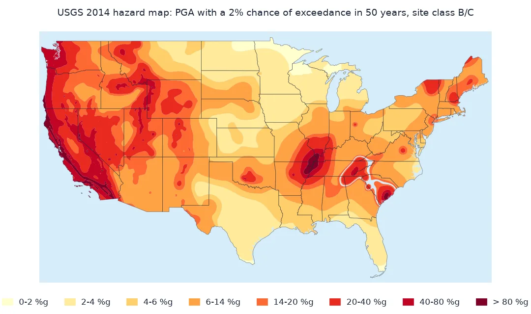
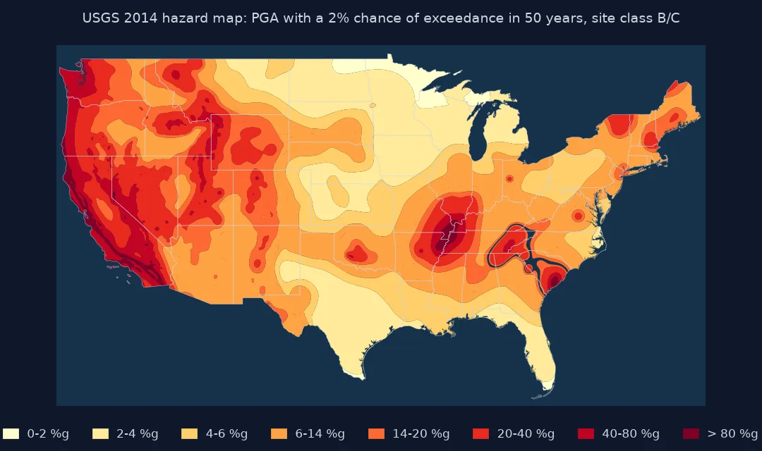
The polygons cover 7.75 million km². The largest band by area is 6–14% of g, 30% of the country. The two highest bands, 40% of g and more, cover 512,000 km², 6.6% of the area, almost all of it in the West, with smaller areas around New Madrid and Charleston.
Repair and dissolve, population by band, counties
1. Repair and dissolve
Polygons from map services are often invalid after generalisation, and one band can be split into many pieces. Check validity, repair with a zero-width buffer, and dissolve by band:
print(f"polygons: {len(H)}; invalid: {(~H.is_valid).sum()}")
H["geometry"] = H.buffer(0)                                   # make_valid() raises on these: mixed-dimension output
print(f"pieces per band: {H.groupby(BAND).size().to_dict()}")
print(f"bands after dissolving: {len(bands)}; all valid: {bands.is_valid.all()}")
polygons: 363; invalid: 46
pieces per band: {'0-2': 2, '14-20': 56, '2-4': 2, '20-40': 66, '4-6': 5, '40-80': 123, '6-14': 47, '> 80': 62}
bands after dissolving: 8; all valid: True
46 of the 363 polygons are invalid as delivered. The band with the most pieces is 40–80% of g, in 123 separate polygons; after repairing and dissolving there is one valid multipolygon per band.
2. Population by hazard band
Assign each county to the band under its representative point and sum the 2023 population estimates:
pts = counties.copy()
pts["geometry"] = counties.representative_point()
joined = gpd.sjoin(pts, bands.reset_index()[[BAND, "geometry"]], predicate="within", how="left")
pop = joined.groupby(BAND).pop2023.sum().reindex(ORDER)
print((pop / 1e6).round(1).rename("millions").to_string())
print(f"counties without a band: {joined[BAND].isna().sum()}; population {joined.loc[joined[BAND].isna(), 'pop2023'].sum():,}")
print(f"people in counties at 40% of g or more: {pop.loc[['40-80', '> 80']].sum() / 1e6:.1f} million ({pop.loc[['40-80', '> 80']].sum() / pop.sum():.0%})")
dspga250_15M.PERCENT_G
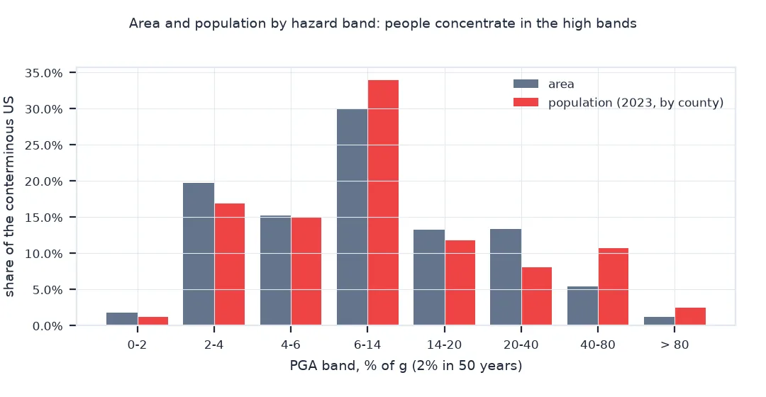
0-2 3.9
2-4 55.7
4-6 49.0
6-14 111.8
14-20 38.8
20-40 26.4
40-80 35.2
> 80 8.0
counties without a band: 43; population 4,058,015
people in counties at 40% of g or more: 43.2 million (13%)
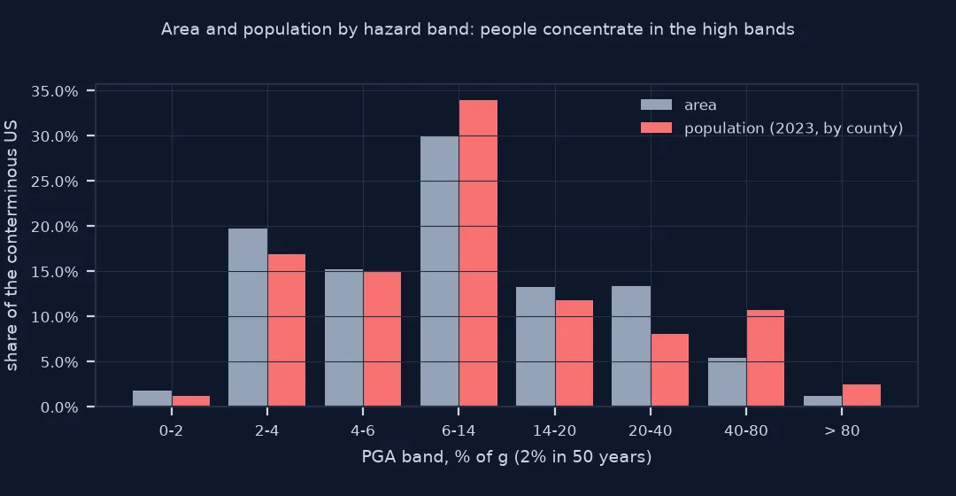
43.2 million people, 13% of the population, live in counties at 40% of g or more, against 6.6% of the area: high hazard and large cities coincide on the West Coast. 43 counties with 4.1 million people fall outside every polygon of this generalised layer. They are not coastal slivers: they include inland counties such as Greenville, South Carolina, and Buncombe, North Carolina, so the gaps are in the 1:15 million geometry itself, visible on the map below as a pale gap in the south-east, and a finer layer would assign them.
3. Which counties
List the most populous counties in the two highest bands:
high = joined[joined[BAND].isin(["40-80", "> 80"])].nlargest(10, "pop2023")
print(high[["CTYNAME", "STNAME", BAND, "pop2023"]].to_string(index=False))
CTYNAME STNAME dspga250_15M.PERCENT_G pop2023
Los Angeles County California 40-80 9663345
San Diego County California 40-80 3269973
Orange County California 40-80 3135755
Riverside County California 40-80 2492442
King County Washington 40-80 2271380
Santa Clara County California > 80 1877592
Alameda County California > 80 1622188
Salt Lake County Utah 40-80 1185813
Contra Costa County California > 80 1155025
Pierce County Washington 40-80 928696
The most populous county in the high bands is Los Angeles, with 9.7 million people, followed by San Diego, Orange and Riverside. King County, Washington, home to Seattle, is fifth. Santa Clara, Alameda and Contra Costa counties around San Francisco Bay are in the highest band, more than 80% of g.
States with the most people in high-hazard counties
The data used on this page
The 2014 USGS national seismic hazard map of PGA with 2% probability of exceedance in 50 years for site class B/C, as the 1:15 million polygons of its map service; the Census Bureau's 2023 county cartographic boundaries (1:20 million) and county population estimates (Vintage 2023).
from pathlib import Path

import geopandas as gpd
import pandas as pd
import requests

Path("data").mkdir(exist_ok=True)
def cached(path, url, **params):
    p = Path(path)
    if not p.exists():
        r = requests.get(url, params=params, timeout=600)
        r.raise_for_status()
        p.write_bytes(r.content)
    return p
BAND = "dspga250_15M.PERCENT_G"
ORDER = ["0-2", "2-4", "4-6", "6-14", "14-20", "20-40", "40-80", "> 80"]
H = gpd.read_file(cached("data/uspga250_2014_15M.geojson", "https://earthquake.usgs.gov/arcgis/rest/services/haz/USpga250_2014/MapServer/102/query",
                         where="1=1", outFields="*", returnGeometry="true", maxAllowableOffset="0.01", f="geojson"))
bands = H.assign(geometry=H.buffer(0)).dissolve(BAND).reindex(ORDER)
counties = gpd.read_file(cached("data/cb_2023_us_county_20m.zip", "https://www2.census.gov/geo/tiger/GENZ2023/shp/cb_2023_us_county_20m.zip")).to_crs(4326)
est = pd.read_csv(cached("data/co-est2023-alldata.csv", "https://www2.census.gov/programs-surveys/popest/datasets/2020-2023/counties/totals/co-est2023-alldata.csv"),
                  encoding="latin-1", dtype={"STATE": str, "COUNTY": str})
est = est[est.SUMLEV == 50].assign(GEOID=lambda d: d.STATE + d.COUNTY)[["GEOID", "STNAME", "CTYNAME", "POPESTIMATE2023"]]
counties = counties.merge(est.rename(columns={"POPESTIMATE2023": "pop2023"}), on="GEOID")
conus = ~counties.STATEFP.isin(["02", "15", "72"])
counties = counties[conus].reset_index(drop=True)
print(f"hazard polygons {len(H)} in {H[BAND].nunique()} bands; {len(counties):,} counties in the conterminous US, {counties.pop2023.sum() / 1e6:.1f} million people")
hazard polygons 363 in 8 bands; 3,109 counties in the conterminous US, 332.7 million people
The service returns 363 polygons in 8 bands. The conterminous US has 3,109 counties and county equivalents with 332.7 million people in the 2023 estimates.
Example 1: states with the most people in high-hazard counties
Sum the population of counties at 40% of g or more by state:
by_state = joined[joined[BAND].isin(["40-80", "> 80"])].groupby("STNAME").pop2023.sum().sort_values(ascending=False)
print((by_state.head(6) / 1e6).round(2).rename("millions").to_string())
print(f"states with any county at 40% of g or more: {len(by_state)}")
STNAME
California 30.26
Washington 5.10
Utah 2.18
Tennessee 1.71
Oregon 1.24
South Carolina 0.89
states with any county at 40% of g or more: 14
California accounts for 30.3 million of the 43.2 million. Washington, Utah, Tennessee, Oregon and South Carolina follow; the eastern two reflect the New Madrid and Charleston source zones. Fourteen states have at least one county at 40% of g or more.
A hazard map summarises thousands of curves
The national hazard map is a contoured summary of thousands of hazard curves: at each point of a fine grid, the PGA whose annual exceedance rate is 1/2,475, contoured into bands. The bands are wide, 40 to 80% of g is a factor of two, so the map is for comparing places, not for designing a building on one of them; that uses the site's own hazard curve or the code's design maps. The edition matters too: the 2014 map is superseded by the 2018 and 2023 models, whose values differ in places, and this page uses 2014 because its polygons are published through a map service.
Counting exposure with a polygon layer and administrative units is a choice between precision and simplicity. Assigning each county to the band at its representative point is simple and keeps county totals intact, but a large county spanning several bands is counted in one; intersecting counties with bands and splitting population by area is more precise only if people are spread evenly, which in western counties they are not. A gridded population layer intersected with the hazard bands would be better still.
Equal-area CRSs, invalid polygons and site class
- Equal-area CRS: area in EPSG:4326 is in square degrees; EPSG:5070, the conterminous US Albers equal-area projection, gives square metres.
- Invalid polygons: generalised service geometries often self-intersect; repair them before dissolving or overlaying. Here
make_valid()fails with a mixed-dimension error andbuffer(0)works; check the repaired area against the original. - Units: the bands are in percent of g; the hazard curve service gives g. See the PGA units fix.
- Site class: the map is for site class B/C; soft soils can raise long-period shaking far more than the map suggests.
Internal links
- How to get seismic hazard curves in Python — the curves behind the map
- Seismic hazard explained — return periods and probabilities
- How to read a USGS ShakeMap and find who was shaken — exposure to one earthquake instead of all possible ones
FAQ
Where can I download the US seismic hazard map as GIS data?
The 2014 maps are available as polygons from the USGS ArcGIS map service; newer models are published as gridded data on ScienceBase.
How many Americans live in high seismic hazard areas?
By the 2014 map and 2023 county estimates, 43.2 million people, 13% of the conterminous US, live in counties whose representative point is at 40% of g or more for 2% in 50 years; 30.3 million of them in California.
What does 40% g with 2% in 50 years mean?
That peak ground acceleration of 0.4 g or more has a 2% chance of being exceeded at least once in 50 years.
Why use an equal-area projection?
Because area in a geographic CRS is in square degrees, which shrink towards the poles; an equal-area projection gives true areas.